Traffic light chase

Question:

You find yourself engaged in a car chase, but it differs from the movies in one key way: Both you and the car that’s chasing you obey all traffic laws, being sure to stop at any and all red lights.

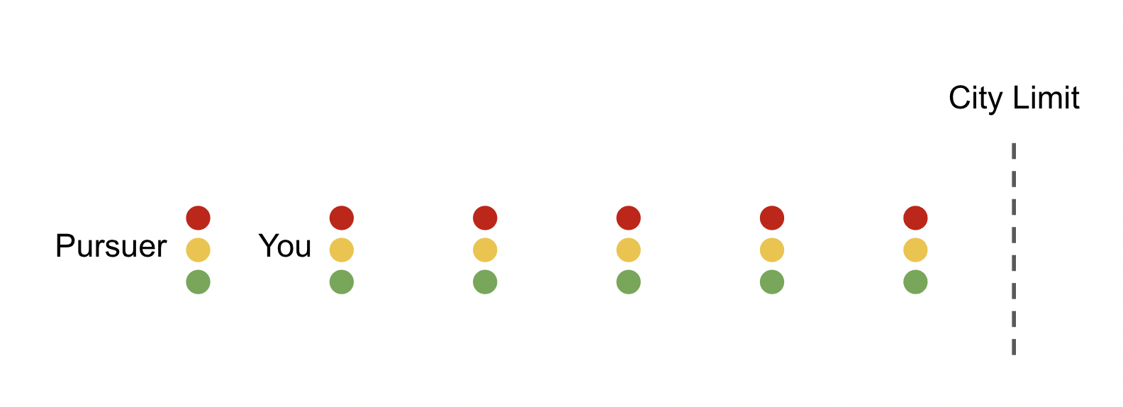
You’re trying to make it to the city limit, but you’re currently one block ahead of your pursuer. Right now you’re both at a red light. The light turns green at the same time for both of you, at which point both cars begin moving east at a speed of one block per minute.

Every time that you come to an intersection, there’s a 50 percent chance the light is green, in which case you coast right on through. But there’s also a 50 percent chance the light is red, in which case it takes exactly one minute for the light to turn green again. These same probabilities govern your pursuer—at each intersection, they have a 50 percent chance of encountering a green light and a 50 percent chance of encountering a red light and having to wait one minute, entirely independent of whatever you might have encountered at that same intersection.

Including the light at which you are now stopped, there are five traffic lights between you and the city limit, as illustrated below. That means there are six lights for your pursuer.

You are displayed as being five stop lights west of the city limit. Your pursuer is six stop lights west of the city limit. How likely is it that you’ll make it past the city limit without being caught?

(Fiddler on the proof)

Solution

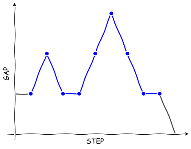
Taken together, the lead and chase car can either move further apart (green light for lead car, red light for chase car), move closer together (red light for lead car, green light for chase car) or remain the same distance apart (same light color for both cars).

If the two cars are going to meet for the first time at step $T$ then, the two cars can do anything in between the first and last step so long as they don’t occupy the same position.

For simplicity, we’re going to change the convention so that the first step happens after the first dual green light, and the final step is just before the cars come together. These moves are obligatory and, so, don’t vary as we consider all possible paths.

Here is one such path:

An example Dyck path, interspersed with stationary moments. Figure thoughtfully prepared by Goh Pi Han with Comic Sans MS.

If we remove the stationary moments where the cars maintain the same relative position, this is just a Dyck path – a path that goes from the bottom left corner to the top right corner of a square lattice without moving under the diagonal.

In principle, our paths can be anything from a pure Dyck path (all up and down moves) to purely staying in place, followed by coming together at the last moment.

An example by hand

For the case of $3$ steps, we can have the cars

• meet at the first possible opportunity,
• spend one light at the same distance before coming together,
• spend two lights at the same distance before coming together,
• spend three lights at the same distance before coming together, or
• have them move apart, then move back down with one light spent at the same distance (with three possible orders for the neutral light).

This has total probability

of escape.

Extra credit

Simulating the system, a curious thing happens: increasing the length of the simulation increases the expected number of steps:

Usually, we’d expect longer runs to bring the estimate closer to its true value.

What does this mean? It’s a telltale sign that the distribution is fat tailed, and has no true representative value! As we run the simulation for longer and longer, there is a greater likelihood that the process samples deeper into the tail, pulling the average up. The longer we sample for, the greater the average… on average.

Finding the distribution

In general, if the Dyck path takes up $2d$ steps of the path, then the stationary moments will take up $(t - 2d)$ steps.

The number of such paths is then be the number of Dyck paths of length $2d$ plus the number of ways to insert $(t-2d)$ diagonal steps between $2d$ Dyck steps. This is just $(2d+1)\cdot(2d+2)\cdots t/(t-2d)!$ which is $t!/((t-2d)!(2d)!) = \binom{t}{2d}.$

The number of Dyck paths of length $2d$ is given by the Catalan numbers, $D_{2d} = C_d = \frac{1}{d+1}\binom{2d}{d}$.

Now, because stationary and up/down moves have distinct probabilities, we need to account for likelihood of each category of path. With $(t-2d)$ sideways moves and $2d$ up/down moves, plus the obligatory final down move, the probability is $\left(\frac14\right)^{2d+1}\left(\frac12\right)^{t-2d}.$

Which makes the probability of ending in exactly $t$ steps:

which comes to

Now, what we are after is the probability of ending the chase by step $T$ or sooner, which is

which makes the cumulative probability of escape by step $T$

As expected, evaluating $P(\text{escape in}\,T\,\text{steps or less})$ at $T=3$ ($5$ in the original convention) gives us $63/128.$

Evaluations of the $\Gamma$-function are approximately related by $\Gamma\left(x + a\right) \approx \Gamma\left(x\right)x^a$ which means the right side of the cumulative distribution scales as $\left(\frac52 + T\right)^{-\frac12}.$

Integrating the cumulative distribution from $0$ to an upper bound $T$ is proportional to $\sqrt{T}.$ Evidently, there is no mean, as the simulation suggested.