Question: Among all six divisions in Fiddler League Baseball (with five teams per division), what is the probability that there exist two divisions such that every team in one division has a higher winning percentage than every team in another division?
(Note that this includes cases where multiple divisions are better or worse than others, such as having two divisions that both have higher winning percentages than some third division.)
Solution
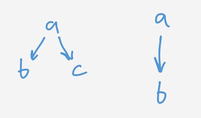
For one division to dominate another, all teams in one need to be better than all the teams in the other. We can represent this by drawing an arrow from $a$ to $b$:

When there are more than two divisions, there is potential for multiple dominance relationships. We could have division $a$ dominate divisions $b$ and $c.$
We could also have a third divison intermingle with two divisions that are in a dominance relationship (e.g. $a$ dominates $b$ but $c$ is neither dominated or dominant). Ordering biggest to smallest, one possible manifestation of this would be
\[a_1 c_1 a_2 b_1 c_2 b_2.\]We can diagram both of these relationships, the first by drawing arrows from $a$ to $b$ and $c$ while the second is simply the original drawing again:
So, a two-division relationship like “A dominates B” can be embedded in more complicated situations involving more than two divisions. This means that when we find the probability of “A dominates B”, we are counting cases where that is the only dominance relationship, as well as every other situation where division “A” dominates division “B”.
So, to properly count the instances where one or more dominance relationships is present, we need to remove double counting.
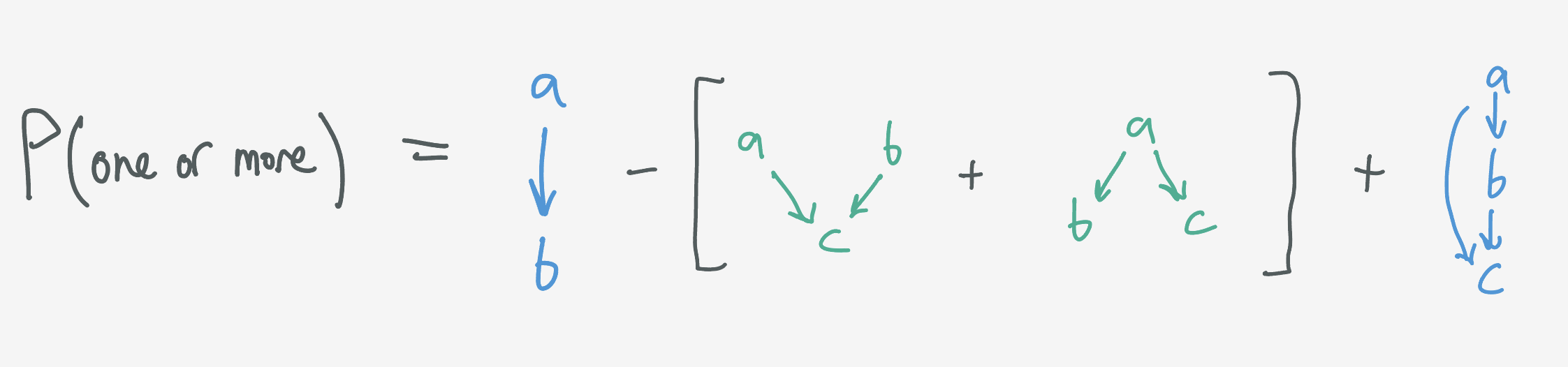
Take the case of $3$ divisions: the probability of one or more dominance relationships is
\[\begin{align} P(\text{one or more}) &= P(\text{one domination}) - P(\text{two dominations}) + P(\text{three dominations}) \\ &= P(\text{one division dominates another}) \\ &\, - \left[P(\text{one division dominates two}) + P(\text{two divisions dominate one})\right] \\ &\, + P(\text{one division dominates another, which dominates another}). \end{align}\]Or, in diagrams:
How to count
How do we find these probabilities?
The key observation is that if we have a dominance relationship between two divisions, it means that their teams separate into non-interacting chunks, like
\[a_1a_2|b_1b_2.\]If that’s the case, then we can shuffle the winning percentages of the teams in each division and the dominance relationships won’t change.
Similarly, if two teams are both dominated by the same team, but don’t necessarily dominate each other, e.g.
\[a_1a_2|b_1c_1c_2b_2,\]then we can do shuffle the teams on either side of the division without changing the dominance relationship.
This tells us all we need in order to find the probabilities.
Example: $a\ \text{dom}\ \{b, c\}$
Suppose there are three divisions where two divisions ($a$ and $b$) dominate a third ($c$) and there are $g$ teams per division.
First, we can assign the division identities (e.g. East, Central, West) to the symbols $a,$ $b,$ and $c$ in $3\times 2\times 1$ ways.
Since divisions $a$ and $b$ are on the same level in the drawing, we can shuffle their teams without changing the dominance relationship. Likewise, we can shuffle the teams in division $c$.
Finally, there is no distinction between $a$ and $b$ (their order is arbitrary), so we divide by $2!$
Together, this makes $3\times 2\times 1(2g)!g!/2!$ ways to order the teams. Since there are $(3g)!$ total ways to order the teams in the league, the probability for two teams to dominate a third is
\[P(\text{two teams dominate one}) = 3\times2\times1\times\frac{(2g)!\times g!}{(3g)!}\frac{1}{2!}.\]Counting rules
That was just one term, but it contains all the crucial ingredients to find a diagram’s probability:
- for each layer with $m$ divisions, multiply by a factor of $(m\times g)!/m!,$ then
- multiply by the number of ways to name the divisions, then
- divide by the total number of orders, $(n\times g)!.$
In general there are many possible dominance relationships. Happily, we can enumerate them by drawing diagrams.
Four divisions
We can use the case of four divisions to do our first calculation. Following the insights about double counting above, we’ll go one level at a time, grouping diagrams by the number of dominance relationships they contain.
With four divisions, the fewest dominations we can have is $0$, and the most is $6$ (if $a$ dominates $b$ dominates $c$ dominates $d,$ we have $3 + 2 + 1 = 6$ total dominations).
To start, there is only one drawing with one domination.
For two dominations, there are three drawings: we can have $a$ and $b$ dominate $c$, $a$ dominate $b$ and $c$, or we can have $a$ dominate $b$ while $c$ dominates $d.$
Plumbing on to the depths of our imagination, we get the following expansion in drawings:
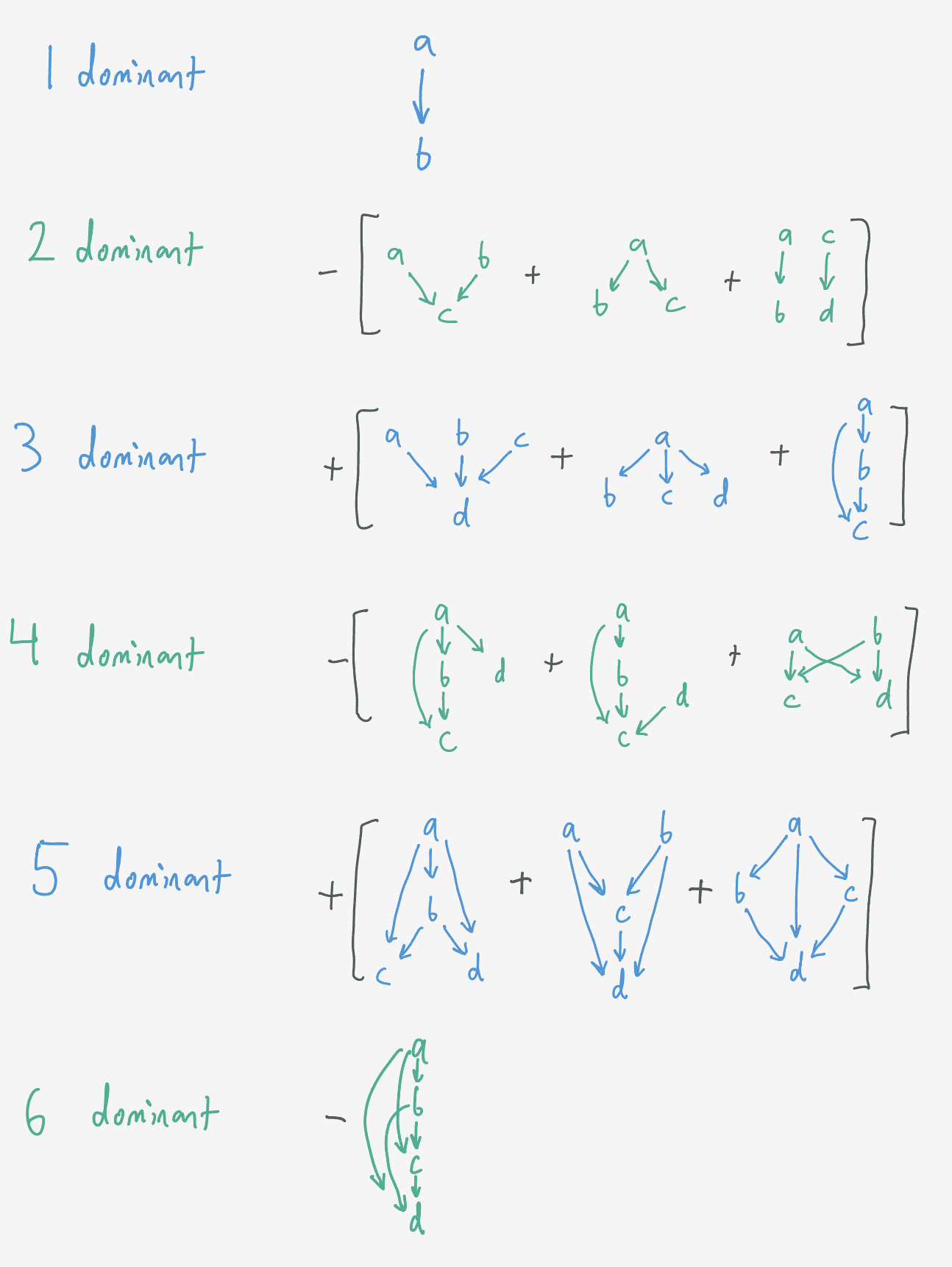
Now, we just have to go term by term and convert these drawings into probabilities.
Most of them follow the rules above in a straightforward way.
For example, the first diagram in the third row has three divisions dominating another: the first layer contributes a factor of $(3g)!/3!,$ the second layer contribues a $g!,$ and there are $4\times 3\times 2$ ways to label the divisions, giving the probability
\[4\times3\times2\frac{(3g)!g!}{(4g)!}\frac{1}{3!}.\]Likewise, the third diagram in the fourth row has two divisions dominating two other divisions. Each layer contributes a factor of $(2g)!/2!$ making the expression
\[4!\left(\frac{(2g)!}{2!}\right)^2\frac{1}{(4g)!}.\]Going through the rest of the drawings and doing the same, we generate the beautiful, shimmering expression
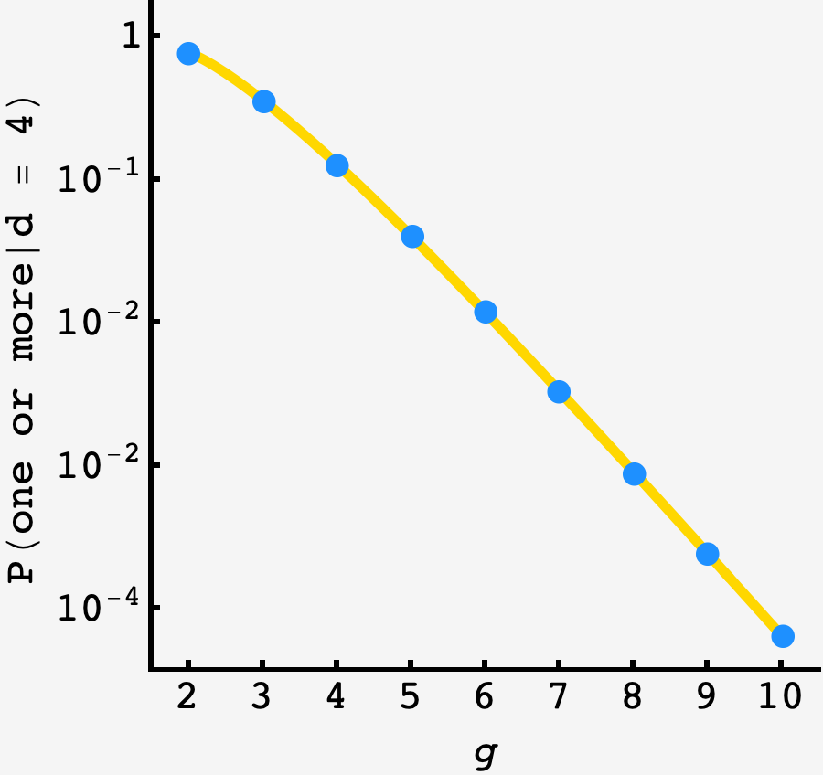
\[\begin{align} P(\text{one or more}|d=4) =\ \ &4\cdot 3\frac{(g!)^2}{(2 g)!} \\ &-\left[4\cdot3\cdot2\frac{g!\cdot (2 g)!}{(3 g)!}\frac{1}{2!} + 4\cdot3\cdot2\frac{g!\cdot (2 g)!}{(3 g)!}\frac{1}{2!} + 4!\left(\frac{g!}{(2 g)!}\right)^2\frac{1}{2!}\right] \\ &+\left[4!\frac{g!\cdot (3 g)!}{(4 g)!}\frac{1}{3!} + 4!\frac{(3 g)!\cdot g!}{(4 g)!}\frac{1}{3!} + 4\cdot3\cdot2\frac{\left(g!\right)^3}{(3 g)!}\right] \\ &-\left[4!\frac{\left((2g)!\right)^2}{(4 g)!}\frac{1}{(2!)^2} + 4!\frac{\left(g!\right)^3}{(4 g)!}\frac{(2g)!}{g!}\frac{1}{2!} + 4!\frac{\left(g!\right)^3}{(4 g)!}\frac{(2g)!}{g!}\frac{1}{2!} \right] \\ &+\left[4!\frac{(2g)!\cdot g!\cdot g!}{(4 g)!}\frac{1}{2!} + 4!\frac{g!\cdot g!\cdot (2g)!}{(4 g)!}\frac{1}{2!} + 4!\frac{g!\cdot (2g)!\cdot g!}{(4 g)!}\frac{1}{2!}\right] \\ &-4! \frac{(g!)^4}{(4g)!}. \end{align}\]Plotting it against an $N=10^7$ round simulation, we see good agreement:
On to the main event.
Six divisions
In principle, we ought to generate a new expansion for $d = 6,$ since more exotic arrangements are possible. However, it isn’t necessary as inspection reveals.
Our series for four divisions is numerically dominated by the two- and three-division terms. This is because it’s rare to achieve the sorts of orderings necessary to have the higher order domination relationships. To take an extreme example, the case of six dominations with four divisions amd three teams per division is only achieved if the winning percentages are ordered like
\[aaabbbcccddd.\]As we add more divisions to the mix, the chance of forming these sorts of intricate chunkings is low.
This argument does not hold when $g$ is one or two, and we should still expect the exotic arrangements to contribute there.
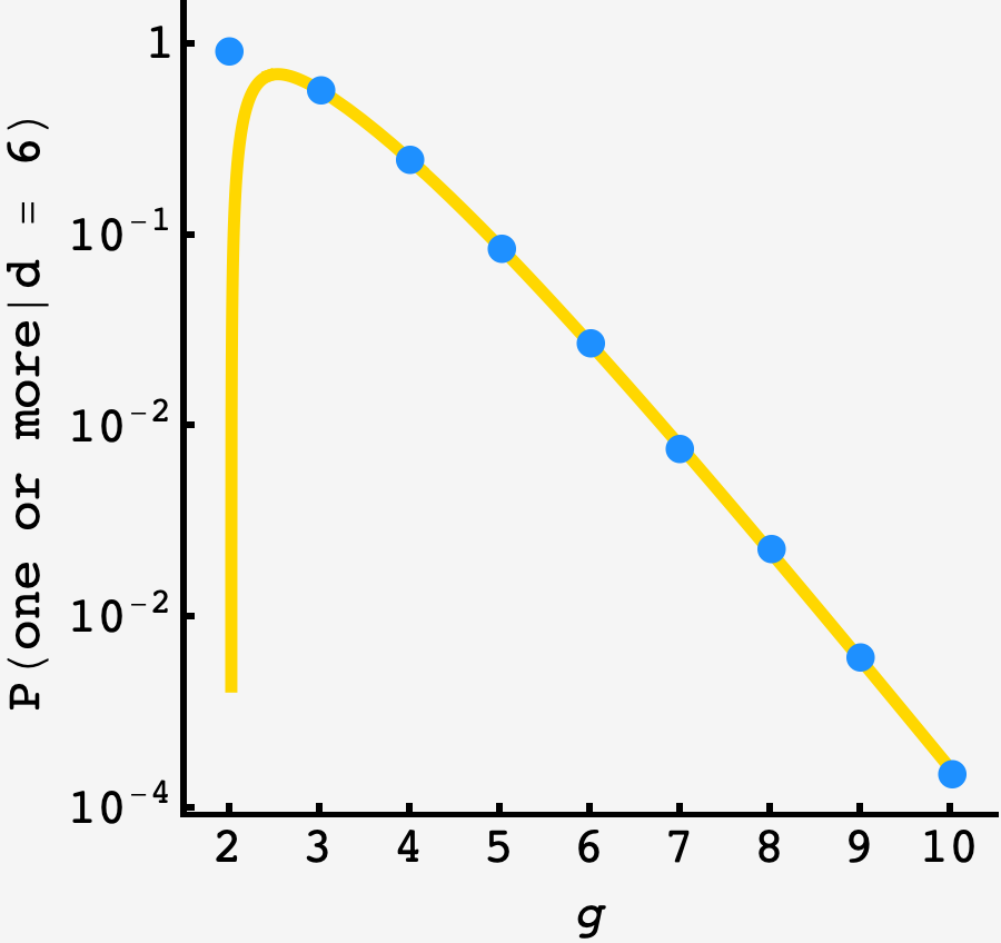
The disappearance of these terms is determined by the value of the ordering factors. For example, one new term corresponds to five divisons getting dominated by one, and has a factor
\[\frac{(5g)!\cdot g!}{(6g)!}\frac{1}{5!}.\]Quickly, this plummets to orders of magnitude below the overall probability. By $g=3$ its value is $2\times10^{-5}$ while the probability is still on the order $1$. In general, higher order terms that are simply extensions of lower order terms (like this five way “fan”) make the greatest contributions, and even they are rare.
With that said, the only change we need to make to our four division expansion is to adjust the counting factors such as $4\times 3\times 2$ to $6\times5\times4.$
Plotting the prediction against an $N=10^6$ round simulation we see that the ignorance of exotic contributions bites us for $g=2$ teams per division, as expected, but by $g=3$ the prediction is within $1\%$ of the simulation.