Question: The Fiddler Baseball League consists of exactly two teams of equal skill: the Algebraists and the Geometers. Over the course of a season, these two teams play each other 162 times. Each team has an equal chance of winning each game, and the results of games are independent of one another.
At the end of the season, on average, how many games would you expect the team with the better record to have won? (If the teams have the same record, then you should include one of them in your calculation.)
Extra credit: After some expansion, the Fiddler Baseball League now boasts 30 teams. Over the course of a season, each team plays each other team five times. (Thus, each team plays a total of 145 games.) As before, each team has an equal chance of winning each game, and the results of games are independent of one another.
At the end of the season, on average, how many games would you expect the team with the best record to have won? (If more than one team has the same best record, then you should include one of them in your calculation.)
Solution
Though the games are discrete events, each team plays enough of them that their distribution is pretty well approximated by its continuous counterpart.
Since each team plays $G = 145$ games and has probability $p = \tfrac12$ to win each one, the mean of this distribution is $\mu = \tfrac12 G = 72.5$ wins and the variance is $\sigma^2 = Gp(1-p) = \tfrac14 \cdot 145 = 36.25$ wins squared.
With this in hand, our plan will be to
- approximate the win total for each team by the normal distribution with matching mean $\mu$ and variance $\sigma^2$
- find the probability that all but one of the win totals is less than $w_\text{max}$
- use that to find the expected value of $w_\text{max}$
In doing this, we’ll run into a nasty integral of CDFs raised to a high power that we will get around through tasteful approximation.
Normalized teams
Since the number of games is large, we can approximate the distribution as a binomial with the same mean and variance $\phi(y) = \mathcal{N}(y\rvert \mu, \sigma).$ So, we can write the number of wins as the mean $\mu$ plus a random normal variable $y_i$ times the width of the distribution
\[w_i = \mu + \sigma y_i,\]and the expected maximum win count as
\[\max_i w_i = \mu + \sigma \max_i y_i.\]This means we’ll be thinking about the maximum surplus relative to the mean, rather than the maximum win count itself, though they both correspond to the same thing.
Expected maximum
The probability distribution of the maximum surplus $y$ is equal to the probability that $(N-1)$ of the teams win less than the maximum surplus $y$ times the probability that the maximum surplus has value $y$ times $N$ since there are $N$ possible winners.
That is
\[P(\max_i y_i = y) = N\left[\int_{-\infty}^y \text{d}y^\prime \phi(y^\prime)\right]^{N-1} \phi(y).\]For ease of writing, we will call the bracketed integral $\Phi(y),$ so the expected maximum surplus is
\[\begin{align} y_\text{max} &= \int_{-\infty}^\infty \text{d}y\, P(\max_i y_i = y) y \\ &= N\int_{-\infty}^\infty \text{d}y\, \Phi(y)^{N-1}\phi(y) y, \end{align}\]and the expected maximum win count is
\[w_\text{max} = \mu + \sigma\cdot y_\text{max}.\]We can evaluate the integral numerically but, before we do, we have to correct for the difference between the variance for the non-independent baseball league and our approximation by normal variables whose collective mean is free to vary.
Variance correction
The variance of the win total of any given team is $\langle\left(w_i - \overline{w}\right)^2\rangle.$ In the real league, $\overline{w}$ is a constant because every game won by some team is lost by another. But with the normal variables we use to model the win totals, there is no such constraint. This means that there is correlation between the mean and the variables. Writing out the mean, we can see the connection
\[\overline{y} = \frac{y_i + (N-1)y_j}{N},\]where $y_j$ is a shorthand for the $(N-1)$ variables for the other teams. The variance for the normal variables is
\[\begin{align} \langle \left(y_i - \overline{y}\right)^2\rangle &= \langle y_i^2\rangle + \langle \overline{y}^2\rangle - 2\langle y_i\cdot \overline{y}\rangle \end{align}\]- the expectation $\langle y_i^2\rangle$ is just $1$ since it is a normal variable.
- $\langle \overline{y}^2\rangle$ is $\langle \frac1{N^2}\left(\sum_k y_k\right)^2\rangle = \frac1{N^2}\cdot N = 1/N.$
- the expectation $\langle y_i \cdot\overline{y}\rangle$ is just $1/N$ since $y_i$ is only correlated with itself and none of the other $y_j.$
So
\[\begin{align} \sigma^2 &= \langle \left(y_i - \overline{y}\right)^2\rangle \\ &= 1 - 2/N + 1/N \\ &= 1 - 1/N \\ &= (N-1)/N. \end{align}\]This shows that the variance of the simulated league $\sigma^2$ is not $1$ but instead the slightly supressed figure $(N-1)/N.$ To correct for this, we need to boost the variance used in the cdf $\Phi$ and pdf $\phi$ from $1$ to $\sqrt{N/(N-1)}.$ So as to avoid carrying around a factor of $1/\sigma^2 = (N-1)/N)$ around everywhere we go, we can make a change of variables to $z = \sqrt{(N-1)/N} y,$ which makes $\text{d}y = \sqrt{N/(N-1)}\text{d}z.$
The expected maximum win count is therefore
\[w_\text{max} = \mu + \sigma\sqrt{\frac{N}{N-1}} \cdot y_\text{max},\]where the integral for $y_\text{max}$ can now be performed numerically with standard issue normal variables (zero mean, and unit variance).
import numpy as np
import scipy as sp

N = 30

mu = (N - 1) * 5
sigma = np.sqrt(N / 4)

def integrand(z):
    return np.sqrt(N/(N-1)) * N * (0.5 * (1 + sp.special.erf(z / np.sqrt(2))))**(N-1) * sp.stats.norm.pdf(z) * z

y_max, _ = sp.integrate.quad(integrand, -np.inf, np.inf)
w_max = mu + sigma * y_max
It comes out to $\langle w_\text{max} \rangle \approx 85.009$ which closely matches the result of a $100,000$ game simulation, $\approx 84.96$
Analytic approximation
Now let’s see if we can make an analytic approximation for the $y_\text{max}.$ The high power on $\Phi(y)$ will tend to push any potential winner into the tails of the cdf, giving hope for an exponential.
\[y_\text{max} = N\int_{-\infty}^\infty \text{d}y\, \Phi(y)^{N-1}\phi(y) y.\]First of all, $\phi(y)$ is the derivative of $\Phi(y)$ so we can rewrite this as
\[y_\text{max} = \int_{-\infty}^\infty \text{d}y\, \left[\frac{\text{d}}{\text{d}y}\Phi(y)^N\right] y.\]As we said, the large power $(N-1)$ in the integral means that any values of $\Phi(y)$ that aren’t close to $1$ are going to be squashed. So, only values of $y$ for which $\Phi(y)$ is close to $1$ will be able to make a significant contribution to the average. Because $\Phi(y)$ is close to $1,$ $ \overline{\Phi}(y) = 1-\Phi(y) $ will be close to zero. After making this substitution, we get
\[\begin{align} \Phi(y)^N &= \left(1- \overline{\Phi}(y)\right)^N \\ &= \left(1- \frac{N\overline{\Phi}(y)}{N}\right)^N \\ &\approx e^{-N\overline{\Phi}(y)} \end{align}\]Now, $\overline{\Phi}(y)$ is hard to integrate, so we’ll need a way to approximate it. A simple way would be to make a linear approximation about some point $y_0.$ But if we did that, $\overline{\Phi}$ would blow up to well outside of the natural range of $0$ to $1$ as $y$ varied from $y_0,$ making the approximation go haywire as $e^{-N(y-y_0)\overline{\Phi}^\prime(y_0)}$ goes to $\infty$ at the lower end. A better option is to linearly approximate the $\log$ of $\overline{\Phi}(y).$ That way, the approximation continues to vary from $0$ to $1$ like the real $\Phi(y).$
\[\begin{align} \log \overline{\Phi}(y) &\approx \log\overline{\Phi}(y_0) + (y-y_0)\frac{\text{d}}{\text{d}y}\log\overline{\Phi}(y)\bigg\rvert_{y=y_0} \\ &\approx \log\overline{\Phi}(y_0) + (y-y_0)\frac{-\phi(y_0)}{\overline{\Phi}(y_0)} \end{align}\]Now we have to choose the anchor point for the approximation, $y_0.$ The distribution $\Phi(y)^{N-1}\phi(y)$ should peak near $\Phi(y) \approx 1 - 1/N$ since, with $N$ teams, the chance for a team’s surplus $y$ to exceed $y_\text{max}$ should be around $1/N.$ So, we can anchor the expansion at the point $y_0$ where $\overline{\Phi}(y_0) = 1/N$ and
\[\log\overline{\Phi}(y) \approx \log\frac1N - N\phi(y_0)\cdot(y-y_0),\]or
\[\overline{\Phi}(y) \approx \frac1N e^{- N\phi(y_0)\cdot(y-y_0)}.\]Plugging this back in to the integral, we get
\[\begin{align} y_\text{max} &= \int_{-\infty}^\infty\text{d}y\, \left[\frac{\text{d}}{\text{d}y}\Phi(y)^N\right] y \\ &\approx\int_{-\infty}^\infty \text{d}y\, \left[\frac{\text{d}}{\text{d}y} e^{-e^{- N\phi(y_0)\cdot(y-y_0)}} \right]y. \end{align}\]We can clean this up by changing variables to $z = N\phi(y_0)\cdot(y-y_0)$ so that $\text{d}z = N\phi(y_0)\,\text{d}y$ and $y = \frac{z}{N\phi(y_0)} + y_0.$
Plugging those in leads us to
\[\begin{align} y_\text{max} &= \int_{-\infty}^\infty \text{d}y\, \left(\frac{z}{N\phi(y_0)} + y_0\right) \frac{\text{d}z}{\text{d}y}\frac{\text{d}}{\text{d}z} e^{-e^{-z}} \\ &= \int_{-\infty}^\infty \text{d}z\, \left(\frac{z}{N\phi(y_0)} + y_0\right) \frac{\text{d}}{\text{d}z} e^{-e^{-z}} \\ &= \frac{z}{N\phi(y_0)}\int_{-\infty}^\infty \text{d}z\, z \frac{\text{d}}{\text{d}z} e^{-e^{-z}} + y_0\int_{-\infty}^\infty \text{d}z\, \frac{\text{d}}{\text{d}z} e^{-e^{-z}} \end{align}\]The second integral just becomes $y_0$ and the first becomes
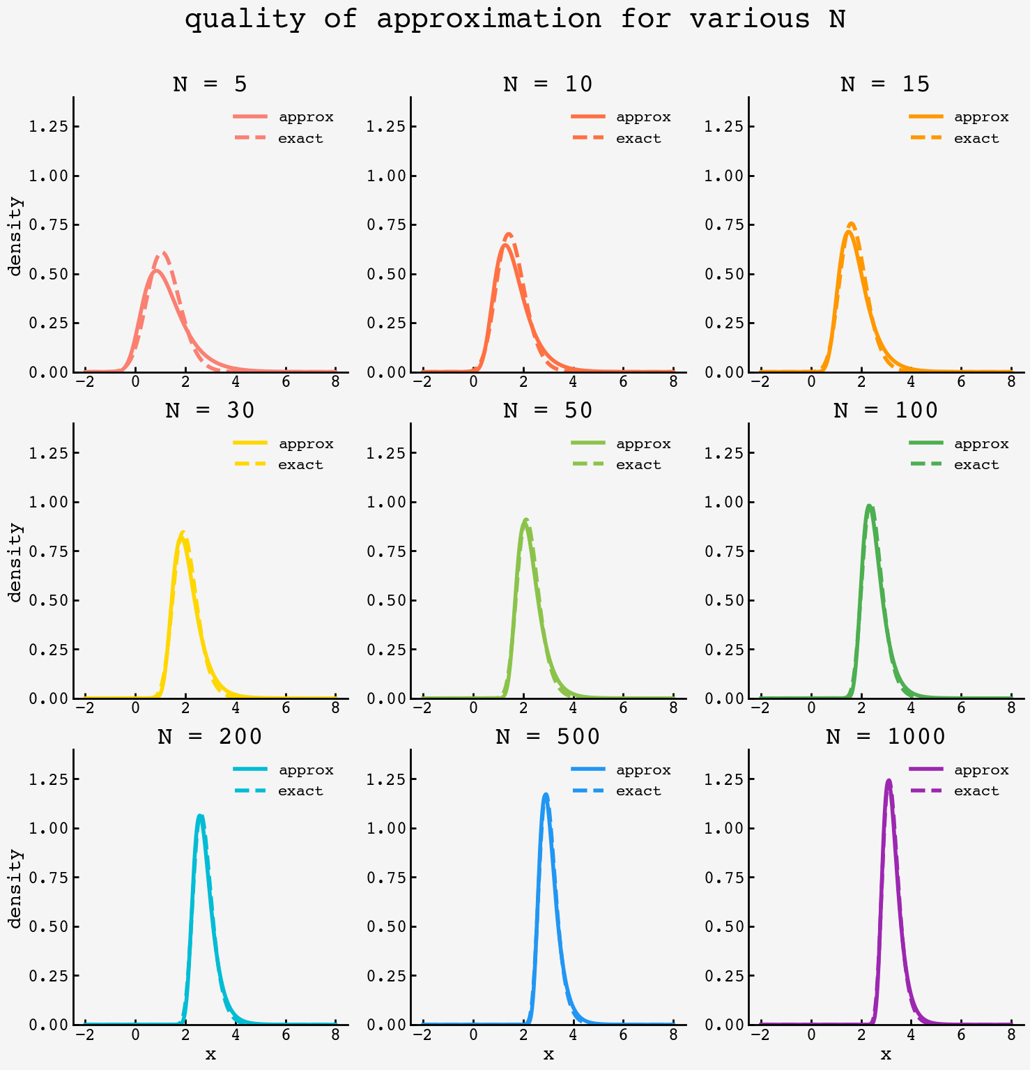
\[\frac{1}{N\phi(y_0)} \int_{-\infty}^\infty \text{d}z\, z \, \overbrace{e^{-z}e^{-e^{-z}}}^\text{Gumbel dist.}.\]which features the Gumbel distribution. The approximation of the pdf and the exact original are shown below for increasing values of $N$:
The first integral comes out to $\gamma/(N\phi(y_0)) $ where $\gamma$ is the Euler-Mascheroni constant, so
\[y_\text{max} = y_0 + \frac{\gamma}{N\phi(y_0)}.\]We picked $y_0$ to that $\Phi(y_0) = 1-1/N$ so $y_0 = \Phi^{-1}(1-1/N).$ For the case of $N = 30$ this gets $\langle w_\text{max}\rangle \approx 85.32,$ which is within $0.4\%$ of the simulated answer.
To see how the winner stands out from the crowd as the number of teams grows, holding to the pattern that each team plays $5$ games against each other team, so that $G=5(N-1),$ we can plot the result as a winning percentage along with a $500,000$ trial simulation and the numerical integral. We see excellent agreement as the number of teams grows.
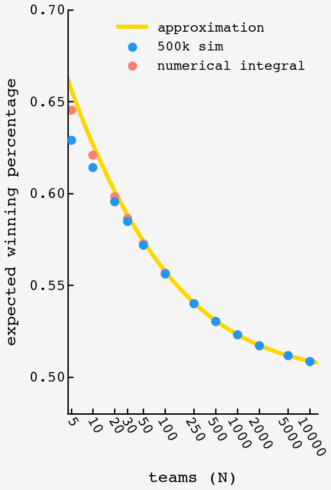
We also see that, somewhat counterintuitively, the best team gets worse and worse as the competition intensifies. Even though there are more oponents to overcome, the crushing regularity of a large number of coin flips means that all teams are stuck close to the mean. As the number of teams grows toward infinity, the expected maximum decays toward $50\%.$
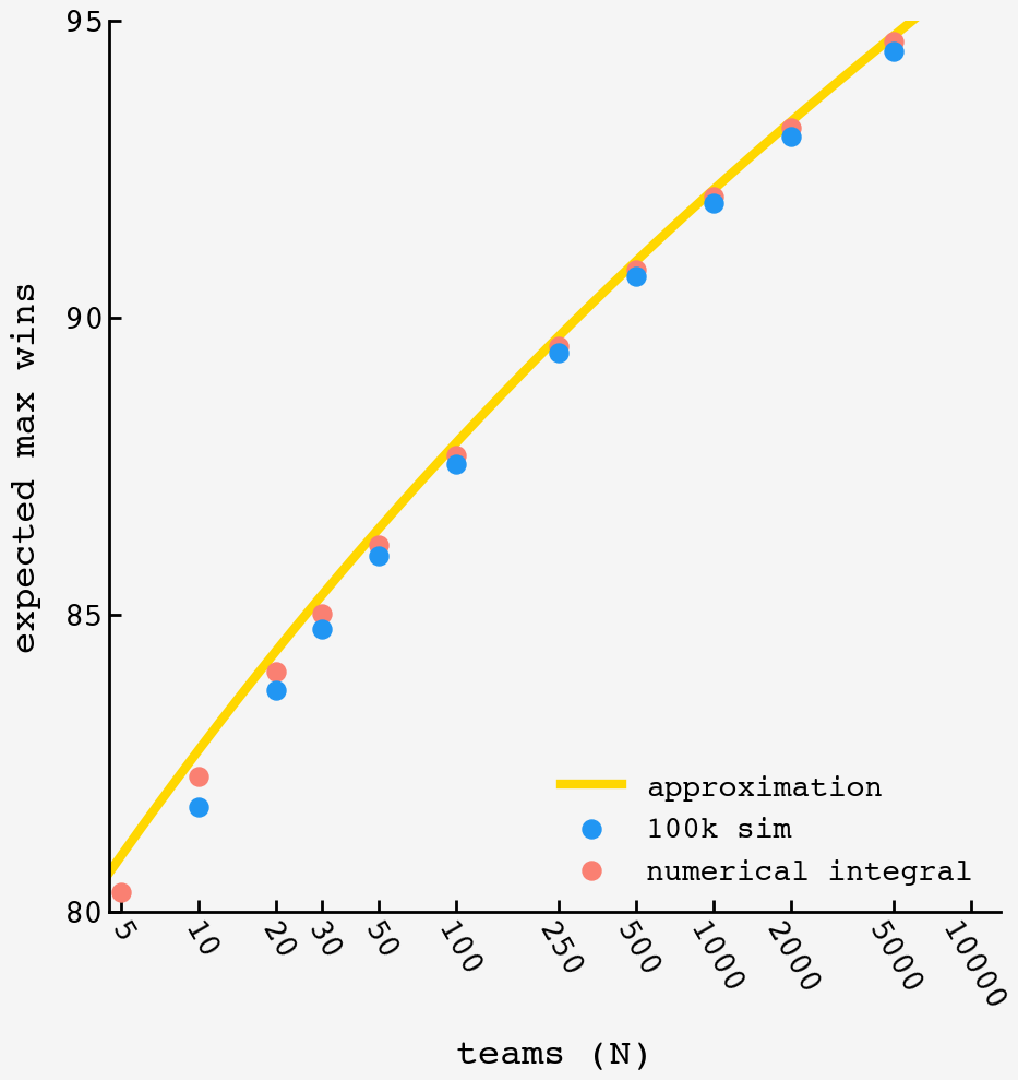
If, instead, we scale the number of teams, but hold the number of games played constant at $145,$ we do indeed see the winning teams win total grow with $N$ though rather slowly. Also, the fidelity of the normal approximation no longer increases with scale since that is tied to the number of games.