Question: Frankie has stored all of her food on lily pad A. However, her food has a tendency to “fly” away. Every second, the food that’s on every lily pad splits up into six equal portions that instantaneously relocate to the six neighboring pads.
At zero seconds, all the food is on lily pad A. After one second, there’s no food on pad A, and $1/6$ of the food is on each of the surrounding six pads. After two seconds, $1/6$ of the food is again on pad A, while the rest of the food is elsewhere.
After how many seconds $N$ (with $N > 2$) will pad A have less than $1$ percent of its original amount?
Solution
Originally, I was not going to write anything up because I just had a recursion I’d evaluated on the computer. But a day later, I realized there ought to be a clean solution through Fourier decomposition. As it turns out, it’s a nice example to learn on, and perhaps generalize for the first time from the textbook example of a simple $1$d random walk.
First, a word about the intuition. Different from transforming a signal that varies in time into a sum of frequency modes, we are not decomposing the probability distribution into signals. Instead, we are transforming the spatial variation into a sum of static patterns. The component patterns are periodic and range in wavelengths all the way from infinity down to the unit spacing of the lattice.
Traditional $1$d random walk
To start, let’s do the ordinary, balanced random walk.
Each lattice point is connected to its two neighbors with equal chance to move left or right at each step. This means that the probability to be at position $x$ at time $t,$ $\omega(x,t)$ is equal to
\[\omega(x,t) = \frac12\omega(x-1,t-1) + \frac12\omega(x+1,t-1).\]Using the fourier transform $\widetilde{\omega}(k,t) = \int_\text{all}\, \text{d}x\, e^{ikx} \omega(x,t)$ we get
\[\begin{align} \widetilde{\omega}(k,t) &= \frac12\int_\text{all}\text{d}x \left[e^{ikx}\omega(x-1,t-1) + e^{ikx}\omega(x+1, t-1)\right] \\ &= \frac12\int_\text{all}\text{d}x \left[e^{ik}e^{ik(x-1)}\omega(x-1,t-1) + e^{-ik}e^{ik(x+1)}\omega(x+1, t-1)\right] \\ &= \frac12\left(e^{ik} + e^{-ik}\right)\widetilde{\omega}(k, t-1) \\ &= \cos k \times \widetilde{\omega}(k, t-1) \\ &= \cos^t k \times \widetilde{\omega}(k, 0). \end{align}\]At long times, the integral is dominated by small values of $k$ close to the peak at $0,$ so we can approximate $\cos k$ as $\approx 1 - k^2/2.$
\[\begin{align} \widetilde{\omega}(k,t) &\approx \left(1-k^2/2\right)^t\widetilde{\omega}(k, 0) \\ &\approx e^{-k^2t/2}\widetilde{\omega}(k,0) \\ &= e^{-k^2t/2}. \end{align}\]The second to last line comes from the fact that the initial condition for $\omega$ is $\omega(x,0) = \delta(x)$ so $\widetilde{\omega}(k,0) = \int\text{d}x e^{ikx}\delta(x) = 1.$
To put this back in terms of position, we add up all the standing patterns with the inverse transform:
\[\begin{align} \omega(x,t) &= \frac{1}{2\pi}\int\text{d}k\, e^{-ikx} \widetilde{\omega}(k,t) \\ &= \frac{1}{2\pi}\int\text{d}k\, e^{-ikx - k^2t/2} \end{align}\]We can turn this into a Gaussian integral by shifting the quadratic in the exponent to kill the linear term
\[\frac{k^2t}{2} + ikx = \left(k\sqrt{\frac{t}{2}} + \frac{ix}{\sqrt{2t}}\right)^2 + \frac{x^2}{2t}.\]Plugging this back in, we get
\[\begin{align} \omega(x,t) &= e^{-x^2/2t}\frac{1}{2\pi}\int\text{d}k\, e^{-\left(k\sqrt{t/2} + ix/\sqrt{2t}\right)^2} \\ &= e^{-x^2/2t}\frac{1}{2\pi\sqrt{t}} \int\text{d}k^\prime e^{-{k^\prime}^2/2} \\ &= e^{-x^2/2t}\frac{1}{\sqrt{2\pi t}} \end{align}\]Finally, we have to multiply by $2$ since the random walker is confined to even sites on even time steps and odd sites on odd time steps.
\[\omega(x,t) = e^{-x^2/2t}\sqrt{\frac{2}{\pi t}}.\]Setting $x$ to zero, we get the $1$d analogue of the disappearing food problem, and after $t$ steps, we expect to find the fraction $f = \sqrt{2/\pi t}$ of the original food left at the origin. Plugging in $f = 1/100,$ it would take approximately $t \approx 20,000/\pi \approx 6,366$ steps for the origin to decay that low.
Hexagonal lattice
To tackle the problem on the hexagonal lattice, we have to accommodate a few details. There are two dimensions that the walkers can move in. They can move directly right or left, changing $x$ by $\pm 1,$ or they can move diagonally changing $(x,y)$ by $\left(\pm 1/2, \pm \sqrt{3}/2\right).$
This makes $6$ directions that are picked uniformly, making the recursion equation (subscripting time for ease of reading)
\[\begin{align} \omega_t(x,y) &= \frac16\omega_{t-1}(x+1,y) + \frac16\omega_{t-1}(x-1,y) \\ &+ \frac16\omega_{t-1}(x+\tfrac12,y+\tfrac{\sqrt{3}}{2}) + \frac16\omega_{t-1}(x+\tfrac12,y-\tfrac{\sqrt{3}}{2}) \\ &+ \frac16\omega_{t-1}(x-\tfrac12,y+\tfrac{\sqrt{3}}{2}) + \frac16\omega_{t-1}(x-\tfrac12,y-\tfrac{\sqrt{3}}{2}). \end{align}\]When we treat $x$ and $y$ as continuous variables, and integrate over them, we are undercounting. The discrete probability $\omega(x,y)$ sums to $1,$ but when we integrate, we are locating each lattice point in a unit of area, and the area of that unit is not $1,$ it is $\sqrt{3}/2.$ So, we will have to account for this when we invert the fourier transform.
Now, the static patterns are two dimensional so we need two wave numbers, $k$ and $\ell,$ instead of one. This means that each spatial dimension gets its own wave number/transform variable. The corresponding mode is $e^{ikx}e^{i\ell y},$ and the Fourier coefficients $\widetilde{\omega}_t(k,\ell)$ tell us how much the $(k,\ell)$ pattern contributes to the probability distribution.
By varying $k$ and $\ell$ we can visualize some of these static modes:
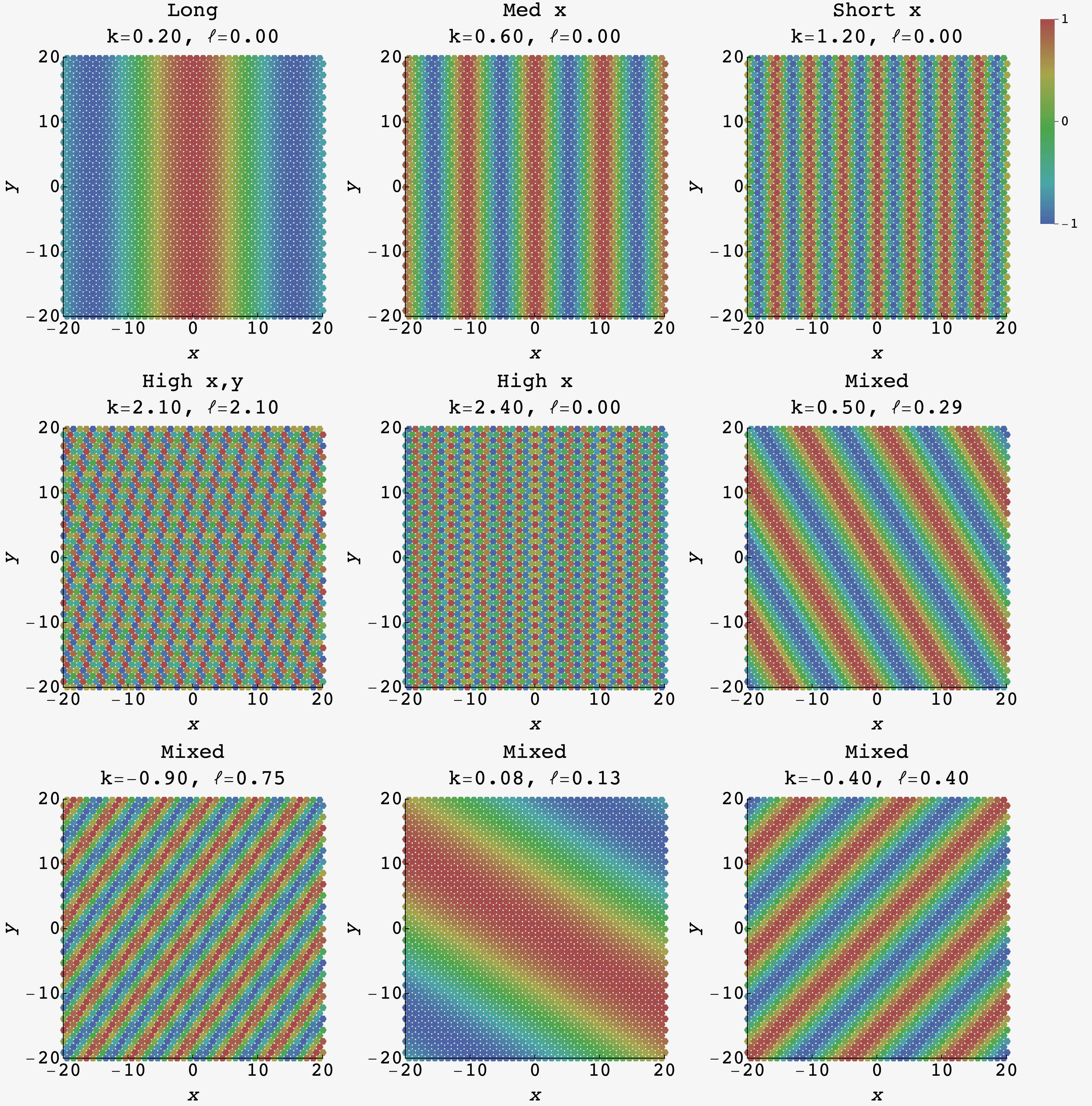
Taking the Fourier transform, we get
\[\widetilde{\omega}_t(k, \ell) = \frac16\int\text{d}x\,\text{d}y\, e^{i{kx+\ell y}} \left[\begin{align}&\omega_{t-1}(x+1,y) + \omega_{t-1}(x-1,y) + \\ &\omega_{t-1}(x+\tfrac12,y+\tfrac{\sqrt{3}}{2}) + \omega_{t-1}(x+\tfrac12,y-\tfrac{\sqrt{3}}{2}) + \\ &\omega_{t-1}(x-\tfrac12,y+\tfrac{\sqrt{3}}{2}) + \omega_{t-1}(x-\tfrac12,y-\tfrac{\sqrt{3}}{2})\end{align}\right].\]Pairing positive and negative complex exponents like we did in the $1$d case, we get a sum of cosines:
\[\begin{align} \widetilde{\omega}_t(k, \ell) &= \frac16\left[e^{-ik} + e^{ik} + e^{-ik/2}e^{-i\sqrt{3}\ell/2} + e^{-ik/2}e^{i\sqrt{3}\ell/2} + e^{ik/2}e^{-i\sqrt{3}\ell/2} + e^{ik/2}e^{i\sqrt{3}\ell/2}\right]\widetilde{\omega}_{t-1}(k, \ell) \\ &= \frac13\left[\cos k + \cos\left(k/2 + \sqrt{3}\ell/2\right) + \cos\left(k/2-\sqrt{3}\ell/2\right)\right]\widetilde{\omega}_{t-1}(k,\ell). \end{align}\]Repeating the expansion, we get a nice product of Gaussians.
\[\begin{align} \widetilde{\omega}_t(k, \ell) &\approx \frac13\left[1-\frac12k^2 + 1 - \frac18k^2 - \frac{3}{8}\ell^2 - \frac{\sqrt{3}}{4}k\ell + 1 - \frac18 k^2 - \frac{3}{8}\ell^2 + \frac{\sqrt{3}}{4}k\ell\right] \widetilde{\omega}_{t-1}(k,\ell) \\ &= \frac13 \left[3 - \frac34 k^2 - \frac{3}{4}\ell^2\right] \widetilde{\omega}_{t-1}(k,\ell) \\ &= \left[1-\frac{1}{4}k^2-\frac14\ell^2\right] \widetilde{\omega}_{t-1}(k,\ell) \\ &= \left[1-\frac{1}{4}k^2-\frac14\ell^2\right]^t \widetilde{\omega}_0(k,\ell) \\ &\approx e^{-\frac{1}{4}k^2t - \frac14\ell^2t} \widetilde{\omega}_0(k,\ell) \\ &= e^{-\frac{1}{4}k^2t - \frac14 \ell^2t} \end{align}\]This means that the hexagonal walk is basically two uncoupled walks in each dimension.
Reconstructing with the inverse Fourier transform we get
\[\begin{align} \omega_t(x,y) &= \frac{1}{\left(2\pi\right)^2} \int\text{d}k\,\text{d}\ell\, e^{-ikx}e^{-i\ell y}\,\widetilde{\omega}_t(k,\ell) \\ &\approx \dfrac{e^{-(x^2+y^2)/t}}{\pi t}. \end{align}\]Again, this undercounts due to $\text{d}x\text{d}y$ being a physical area, so we scale up by the unit area $\sqrt{3}/2$ and get
\[\omega_t(x,y) \approx \frac{\sqrt{3}}{2}\dfrac{e^{-(x^2+y^2)/t}}{\pi t}.\]Watching the distribution over time, the probability starts peaked at the origin and then proceeds outward
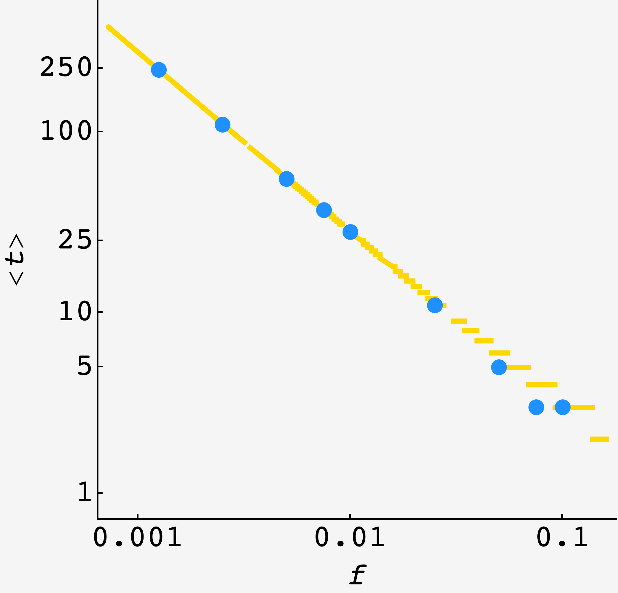
We can plug in $(x,y) = (0,0)$ and solve for the value of $t$ when it equals $f.$ We get
\[t\approx \frac{\sqrt{3}}{2\pi f}.\]This is $\approx 27.57$ for $f = 1/100$ which, after taking the ceiling, is dead on with the exact result of $28.$