Question: You’re in your town’s head to head marble racing championship, the traditional way to determine who is the town’s next mayor. The race is split into two heats and your time in either heat is a random, normally distributed variable. If you have the fastest time in the first run, what is the probability $P_\text{win it all}$ that you end up winning the event, as determined by the sum of your times on heat run?
Extra credit: what if there are $29$ other candidates in the race?
Extra extra credit What about $N$?
Solution (originally published 2021-01-24)
If the first skier wins the first round by $\Delta T_1,$ they will prevail so long as they don’t lose the second round by more than $\Delta T_1.$
The gap between the first round times $\left(\Delta T_1 = t^\text{A}_1 - t^\text{B}_1\right)$ which has some symmetric distribution $P(\Delta T_1).$ Since we know that person $\text{A}$ won the first round, we condition on the left side of $P$ and the expected value of $\Delta T_1$ is whatever the $25^\text{th}$ percentile of the distribution is.
If person $\text{A}$ is to win overall, $\Delta T_1$ has to be less than or equal to $-\Delta T_2.$ The gap in the second round is a random variable from the same distribution, so the chance that $\Delta T_1 < -\Delta T_2$ (and, therefore, that player $\text{A}$ wins) is $P_2 = 1 - 0.25 = 0.75.$
Pushing on
There are several ways to manifest the result above through calculation but none of the them yielded to generalization. An approximate attempt yielded good results for low $N$ but broke down as $N$ grew, notably resisting the stable plateauing that persists near $30\%$ for a wide range of $N.$
A simulation suggests a roughly linear decrease on log-log axes, and yields $P_{30} \approx 0.314409.$ Its overall behavior is decently approximated by $P \approx x^{-1/3}$ over a wide range:
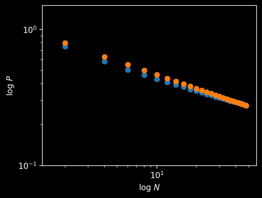
Fig: plot of $\log P(\text{first round winner wins})$ vs $\log N.$
def round(N):

    data = np.random.normal(0, 1, size=N)
    first_win = data.argmin()

    data += np.random.normal(0, 1, size=N)
    overall_win = data.argmin()

    if first_win == overall_win:
        return 1
    return 0
My attempts at an approximate solution for $N=30$ got the right shape, but took too long to “turn up”. Updates forthcoming if I make progress.
2025-11-18 Update
The formal solution I was trying to approximate (to no avail) almost five years ago was the following:
If the first and second heat times for racer $j$ are $f_j$ and $s_j$, and the winner goes first, then
- each $f_j$ can range from $f_1$ up to $\infty$ (all other racers are slower than the winner in heat one)
- each $s_j$ can range from $f_1 + s_1 - f_j$ up to $\infty$ (because anything faster would cause racer $j$ to win the race)
- $f_1$ and $s_1$ can range from $-\infty$ to $\infty$ (because the winner sets the constraints for the other racers)
The probability that racer $j$ meets these conditions is
\[J(f_1,s_j) = \int\limits_{f_1}^\infty \text{d}f_j\, \mathcal{N}(f_j) \int\limits_{f_1 + s_1 - f_j}^\infty \text{d}s_j\, \mathcal{N}(s_j).\]The constraint on the losers is set by the times of the winner, Racer $1$, so they’re independent of each other and the probability that all $(N-1)$ satisfy the constraint is just
\[J(f_1,s_1)^{N-1}.\]The probability that the racer who wins the first heat wins the whole race is then just
\[N \int\limits_{-\infty}^\infty \text{d}f_1\mathcal{N}(f_1) \int\limits_{-\infty}^\infty\text{d}s_1 \mathcal{N}(s_1)J(f_1,s_1)^{N-1}.\]We can evaluate this numerically for e.g. $N=30$ and we get $0.31471089\ldots$, which closely matches simulation.
However, it is not easy to get a formula for general $N$ because the integral $J$ depends strongly on the values of $f_1$ and $s_1$. Depending on how they’re set it could be very likely, a tossup, or very unlikely for a given Racer $j$ to lose to Racer $1$. Without definite values, we can’t evaluate the integral or systematically approximate it.
The crucial insight is that we actually don’t have to…
Instead, we can calculate the expected value of the probability that the winner of the first heat wins the whole race. The strategy will be to find the probability that the winner of the first heat wins in terms of their first heat time, and then average this using the probability distribution of the winning first heat time.
\[P(\text{heat 1 winner wins}) = \int\limits_{-\infty}^\infty \text{d}x\, P(\text{first heat winner wins}|x)P(\text{first heat time is }x).\]We know two useful things about the winner
- they won the first heat
- their first heat time plus their second heat time is less than the expected minimum total time of the $(N-1)$ other racers.
To win the first heat, they need the probability of beating their first heat time $f_1$ to be less than $1/N.$
The probability that a normal variable is less than a target $v$ is
\[P(z < -v) = \int\limits_{-\infty}^{-v} \text{d}z\, \mathcal{N}(z),\]which is approximated by
\[\mathcal{N}(v)/v.\]The minimum should occur at the value $\gamma$ where the probability to fall short of $\gamma$ is less than $\frac1N.$ So, we can find the likely value of $f_1,$ $\gamma,$ by solving
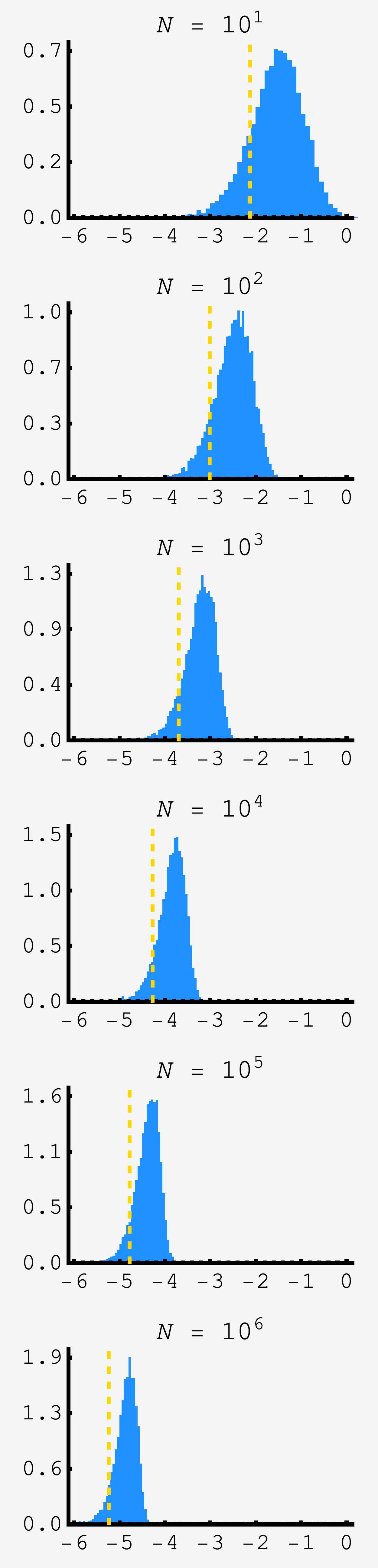
\[\begin{align} \frac{\mathcal{N}(\gamma)}{\gamma} &= \frac1N \\ \frac{e^{-\gamma^2/2}}{\sqrt{2\pi}\gamma} &= \frac1N \\ \gamma^2/2 + \log \sqrt{2\pi}\gamma &= \log N. \end{align}\]We could solve this by iterated approximation, but to first order we can keep the dominant quadratic $\gamma$ term and find $\gamma \approx \sqrt{2\log N}.$ It isn’t the most wonderful approximation, but improves as $N$ grows and is consistent with the other approximations we’ll make. The plot shows the distribution of minima for samples of $N$ unit normal variables in blue and the approximation for the mean in gold for $N$ ranging from $10$ to $10^6.$
$f_1$ will be peaked near $\gamma$, but vary around it. We can rewrite $f_1 = -\gamma + x$ where $x$ is assumed small compared to $\gamma.$ The total time taken is $f_1 + s_1.$ Because $f_1$ and $s_1$ are both normal variables with variance $1$, if we divide the sum by $\sqrt{2}$ it will be a normal variable as too: $(f_1+s_1)/\sqrt{2}.$
Racer $1$ wins if $f_1+s_1$ is less than the smallest time of the $(N-1)$ other racers. The total time for other racers is also a normal variable $t_j = (f_j+s_j)/\sqrt{2}.$ The expected minimum for this variable is found the same way we found it for $f_1,$ except with $(N-1)$ in place of $N.$ In practice, $(N-1)\approx N$ for large $N$ so the expected minimum for the other racers is $-\gamma$ too.
So, Racer $1$ will win if $(f_1+s_1)/\sqrt{2} < -\gamma$ or
\[\frac{-\gamma + x}{\sqrt{2}} + \frac{s_1}{\sqrt{2}} < -\gamma,\]which is equivalent to
\[s_1 < -\overbrace{\left(\sqrt{2}-1\right)}^{\nu}\gamma + x.\]So, for a given value of $x,$ the probability Racer $1$ wins is $\mathcal{N}(\nu \gamma + x)/(\nu\gamma + x).$ Working this out, we get
\[\begin{align} P(\text{Racer 1 wins}|x) &= \frac{1}{\sqrt{2\pi}}\frac{1}{\nu\gamma+x} e^{-(\nu\gamma+x)^2/2} \\ &= \frac{1}{\sqrt{2\pi}}\frac{1}{\nu\gamma+x} e^{-(\nu^2\gamma^2 + 2\nu \gamma x + x^2)/2} \\ &\approx \frac{1}{\sqrt{2\pi}}\frac{1}{\nu\gamma} e^{-(\nu^2\gamma^2 + 2\nu \gamma x)/2} \\ &= \frac{1}{\sqrt{2\pi}}\frac{1}{\nu\gamma} \left(e^{-\gamma^2/2}\right)^{\nu^2} e^{-\nu \gamma x} \\ &= \frac{1}{\sqrt{2\pi}}\frac{1}{\nu\gamma} \left(\frac{\sqrt{2\pi}\gamma}{N}\right)^{\nu^2} e^{-\nu\gamma x} \end{align}\]We dropped the $x^2$ term in the exponent on the assumption that the probability distribution of $x$ will crush the integrand before the $x^2$ term has a big impact. This will not be true for small values of $N$ so we should expect our approximation to overestimate, and converge asymptotically from above.
Now, the probability that a single racer’s first heat time is over $-\gamma + x$ is one minus the probability that they’re under: $1 - \frac{\mathcal{N}(-\gamma + x)}{-\gamma + x}.$ And the probability that none of the $(N-1)$ people’s first heat time is faster is $\left[1 - \frac{\mathcal{N}(-\gamma + x)}{(-\gamma + x)}\right]^{N-1}.$
\[\begin{align} P(\text{first heat time < }-\gamma + x) &= \frac{\mathcal{N}(-\gamma + x)}{(\gamma + x)} \\ &= \frac{1}{\sqrt{2\pi}}\frac{e^{-(-\gamma + x)^2/2}}{(\gamma + x)} \\ &= \frac{1}{\sqrt{2\pi}}\frac{e^{-(\gamma^2 -2x\gamma + x^2)/2}}{(\gamma + x)} \\ &\approx \frac{1}{\sqrt{2\pi}}\frac{e^{-(\gamma^2 -2x\gamma)/2}}{\gamma} \\ &= \frac{\mathcal{N}(\gamma)}{\gamma}e^{\gamma x} \\ &= e^{\gamma x}/N \end{align}\]The probability that a racer’s first heat time is greater than $(-\gamma + x)$ is then $(1-e^{\gamma x}/N)$ and the probability that the minimum first heat time is greater than $(-\gamma+x)$ is $\approx(1-e^{\gamma x}/N)^N = e^{-e^{\gamma x}}.$ So, the cumulative probability that the minimum is less than $(-\gamma+x)$ is $1 - e^{-e^{\gamma x}}$ and the probability distribution that the minimum first heat time is $x$ exactly is then just
\[P(\text{first heat min} = x) = \frac{\text{d}}{\text{d}x} 1 - e^{-e^{\gamma x}} = \gamma e^{\gamma x} e^{-e^{\gamma x}}.\]Putting it all together, the probability that the winner of the first heat wins the entire race is
\[\begin{align} P(\text{heat 1 winner wins}) &= \int\limits_{-\infty}^\infty \text{d}x\, P(\text{first heat winner wins}|x)P(\text{first heat time is }x) \\ &\approx\frac{1}{\sqrt{2\pi}}\frac{1}{\nu\gamma} \left(\frac{\sqrt{2\pi}\gamma}{N}\right)^{\nu^2} \int\limits_{-\infty}^{\infty} \text{d}x\, e^{-\nu \gamma x} \gamma e^{\gamma x} e^{-e^{\gamma x}}. \end{align}\]The integral has no actual $\gamma$ dependence which we can see by setting $z = e^{\gamma x}$ so that $\text{d}z = \gamma e^{\gamma x} \text{d}x = \gamma z \text{d}x$ so that the probability becomes
\[\begin{align} P(\text{heat 1 winner wins}) &\approx \frac{1}{\sqrt{2\pi}}\frac{1}{\nu\gamma} \left(\frac{\sqrt{2\pi}\gamma}{N}\right)^{\nu^2} \int\limits_{0}^{\infty} \text{d}z\, \frac{1}{\gamma z} \gamma z e^{-z} z^{-\nu} \\ &\approx \frac{1}{\sqrt{2\pi}}\frac{1}{\nu\gamma} \left(\frac{\sqrt{2\pi}\gamma}{N}\right)^{\nu^2} \int\limits_{0}^{\infty} \text{d}z\, e^{-z} z^{-\nu}. \end{align}\]The integral will get us an overall numerical factor, but already we can see how the problem will scale with $N.$ Pulling out the $N$ dependent terms from the prefactor, we have
\[\begin{align} P(\text{heat 1 winner wins}) &\propto \gamma^{\nu^2-1}N^{-\nu^2} \\ & \propto (\log N)^{1-\sqrt{2}} N^{-(3-2\sqrt{2})}. \end{align}\]This integral is just the gamma function $\Gamma(1-\nu)$ making the final result
\[\begin{align} P(\text{heat 1 winner wins}) &\approx \frac{1}{\nu}(4\pi)^\frac{\nu^1-1}{2}\Gamma(1-\nu)\left(\log N\right)^{\frac{\nu^2-1}{2}}N^{-\nu^2} \\ &\approx (1+\sqrt{2})(4\pi)^{1-\sqrt{2}}\Gamma[2-\sqrt{2}]\left(\log N\right)^{1-\sqrt{2}} N^{-(3-2\sqrt{2})}. \end{align}\]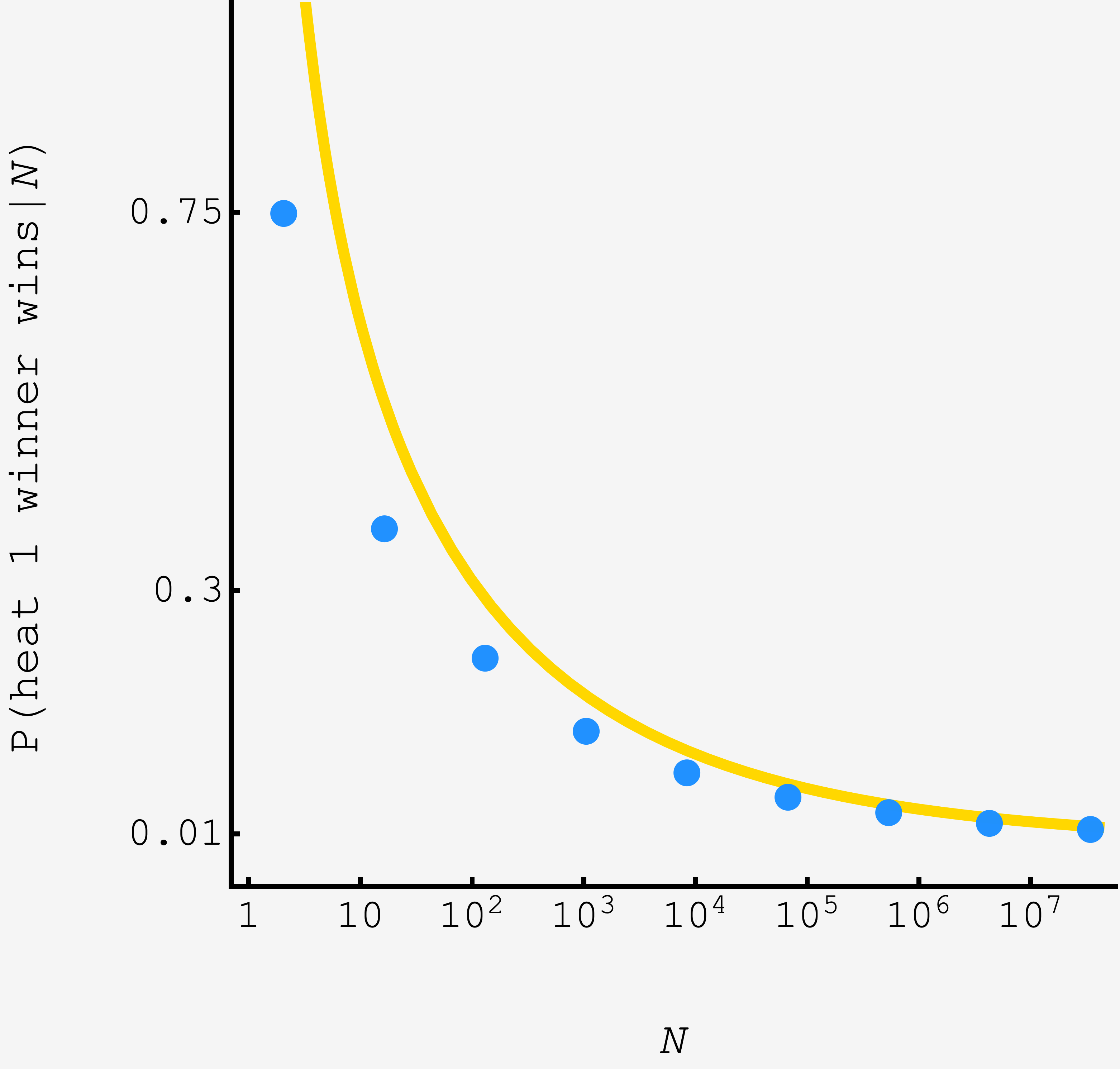
As the number of racers increases the advantage of the first heat winner grows, far exceeding $1/N.$
To get more accurate predictions for small $N,$ we’d need to perturbatively develop the $e^{-x^2/2\gamma^2}$ that we dropped for the approximation, model the fluctuations in the second place racer, and use a higher fidelity estimates for $\gamma.$ The perturbative terms shrink with powers of $1/\log N$, so convergence is slow, but we can already see the asymptotic result (gold curve) and the simulation (blue points) converging.
Update 2025-12-11
The wonders never cease. In this update we’re going to make two of the improvements suggested above:
- modeling the fluctuations of the next best racer
- use the inverse complementary error function to approximate the extrema
In our original scheme to find the approximate value of $\gamma,$ we approximated the integral
\[P(z < -\gamma) = \int\limits_{-\infty}^{-\gamma} \text{d}z\, \mathcal{N}(z)\]by $\mathcal{N}(\gamma)/\gamma,$ set it equal to $1/N$
\[\begin{align} \frac{\mathcal{N}(\gamma)}{\gamma} &= \frac1N \\ \frac{e^{-\gamma^2/2}}{\sqrt{2\pi}\gamma} &= \frac1N \\ \gamma^2/2 + \log \sqrt{2\pi}\gamma &= \log N, \end{align}\]dropped the $\log\sqrt{2\pi}\gamma$ term and solved for $\gamma$ to find $\gamma \approx \sqrt{2\log N}$ and called it a day.
But if we don’t make the integral approximation, we can just write the solution in terms of the complementary error function. After rescaling the variable of integration, the integral is equal to half the error function of $\gamma/\sqrt{2}:$
\[P(z < -\gamma) = \frac12\text{erfc}(\gamma/\sqrt{2}).\]So, the $\gamma$ we are after is $\gamma = \sqrt{2}\text{erfc}^{-1}\left(\frac{2}{N}\right).$
Our original condition for the winner of heat $1$ to win it all pegged the second best racer at constant $-\gamma,$ so we had
\[\frac{f_1+s_1}{\sqrt{2}} < -\gamma.\]However, the minimum of the competition will fluctuate around $-\gamma$ just the winner of heat $1$ does. Accounting for this, we get the new condition
\[\begin{align} \frac{-\gamma + x+s_1}{\sqrt{2}} &< -\gamma + y \\ s_1 &\lt -\nu\gamma + \sqrt{2}y - x. \end{align}\]This makes the probability that the first heat winner wins it all, conditioned on their first heat time $-\gamma + x,$ and the competition’s time $-\gamma + y,$ equal to
\[\begin{align} P(\text{heat 1 winner wins}\rvert x, y) &= \int\limits_{-\infty}^{-\nu\gamma +\sqrt{2}y - x} \text{d}z\, \mathcal{N}(z)\\ &= f(-\nu\gamma + \sqrt{2}y - x). \end{align}\]In the original calculation, we approximated this quantity using $f(z) \approx \mathcal{N}(z)/z,$ which was in part motivated by the fact that we could then take advantage of $e^{-\gamma^2/2} \approx 1/N.$ However, this approximation has low accuracy for small $\gamma$ and since $\gamma$ is logarithmic in $N,$ this is a source of slow convergence. And in any case, with our refined estimate for $\gamma,$ we can’t make that substitution. This time we’re going to preserve $f$ for the bulk and only use the $\mathcal{N}(z)/z$ approximation to extract the the fluctuation.
We assume that the fluctuations around $-\gamma$ are small compared to $\gamma,$ so $\left(x - \sqrt{2}y\right)$ is small compared to $\nu\gamma.$ This means we can approximate $f(-\nu\gamma + \delta)$ in terms of $f(-\nu\gamma).$
Applying the same $\mathcal{N}(z)/z$ approximation, we get
\[\begin{align} f(-\nu\gamma + \delta) &\approx f(-\nu\gamma) \cdot \frac{\mathcal{N}(-\nu\gamma + \delta)}{\mathcal{N}(-\nu\gamma)} \cdot \frac{-\nu\gamma}{-\nu\gamma + \delta} \\ &= f(-\nu\gamma)\cdot \exp\left[{\frac12\nu^2\gamma^2 - \frac12(\nu^2\gamma^2 - 2\nu\gamma\delta + \delta^2)}\right]\cdot \frac{-\nu\gamma}{-\nu\gamma + \delta} \\ &\approx f(-\nu\gamma)e^{\nu\gamma\delta}. \end{align}\]Now, all have to do is put the integral back together. The probability that the winner of heat $1$ wins the race is now an integral over the heat $1$ winner’s heat $1$ time, through $x,$ and the second place racer’s total time, through $y:$
\[\begin{align} P(\text{heat 1 winner wins}) &= \int\limits_{-\infty}^\infty\text{d}x \int\limits_{-\infty}^\infty\text{d}y\, P(\text{heat 1 winner wins}\rvert x, y) \\ &\quad \times P(\text{first heat time is}\, -\gamma + x) P(\text{second place total time is}\, -\gamma + y).\end{align}\]As before, $P(x) \approx \gamma e^{\gamma x}e^{-e^{\gamma x}}$ and now $y,$ being the minimum of nearly as many random normal variables, is also distributed like $P(y) \approx \gamma e^{\gamma y}e^{-e^{\gamma y}},$ so we get
\[\begin{align} P(\text{heat 1 winner wins}) &= \int\limits_{-\infty}^\infty\text{d}x \int\limits_{-\infty}^\infty\text{d}y\, f(-\nu\gamma)e^{\nu\gamma \sqrt{2}y}e^{-\nu\gamma x}\gamma^2 e^{\gamma x}e^{-e^{\gamma x}} e^{\gamma y}e^{-e^{\gamma y}} \\ &= f(-\nu\gamma)\int\limits_{-\infty}^\infty\text{d}x e^{-\nu\gamma x}\gamma^2 e^{\gamma x} e^{-e^{\gamma x}}\int\limits_{-\infty}^\infty\text{d}y\, e^{\nu\gamma \sqrt{2}y} e^{\gamma y}e^{-e^{\gamma y}}. \end{align}\]The $x$ and $y$ integrals are versions of the integral in our original calculation. Applying the same pattern, and re-expressing $f$ in terms of the complementary error function, we get
\[\begin{align} P(\text{heat 1 winner wins}) &\approx f(-\nu\gamma)\Gamma(1-\nu)\Gamma(1 + \sqrt{2}\nu) \\ &= \frac12 \text{erfc}\left[\frac{(\sqrt{2}-1)\gamma}{\sqrt{2}}\right]\Gamma(2-\sqrt{2})\Gamma(3-\sqrt{2}) \\ &= \text{erfc}\left[\left(\sqrt{2}-1\right)\text{erfc}^{-1}\left[\frac{2}{N}\right]\right]\frac{2-\sqrt{2}}{2}\Gamma(2-\sqrt{2})^2 . \end{align}\]Before we graph it, let’s take stock of its features.
Aesthetically, it seems like a clear win. On grounds of transparency, it depends on your intuition with the error function. However, on the most important ground of accuracy, it’s an unmitigated triumph:
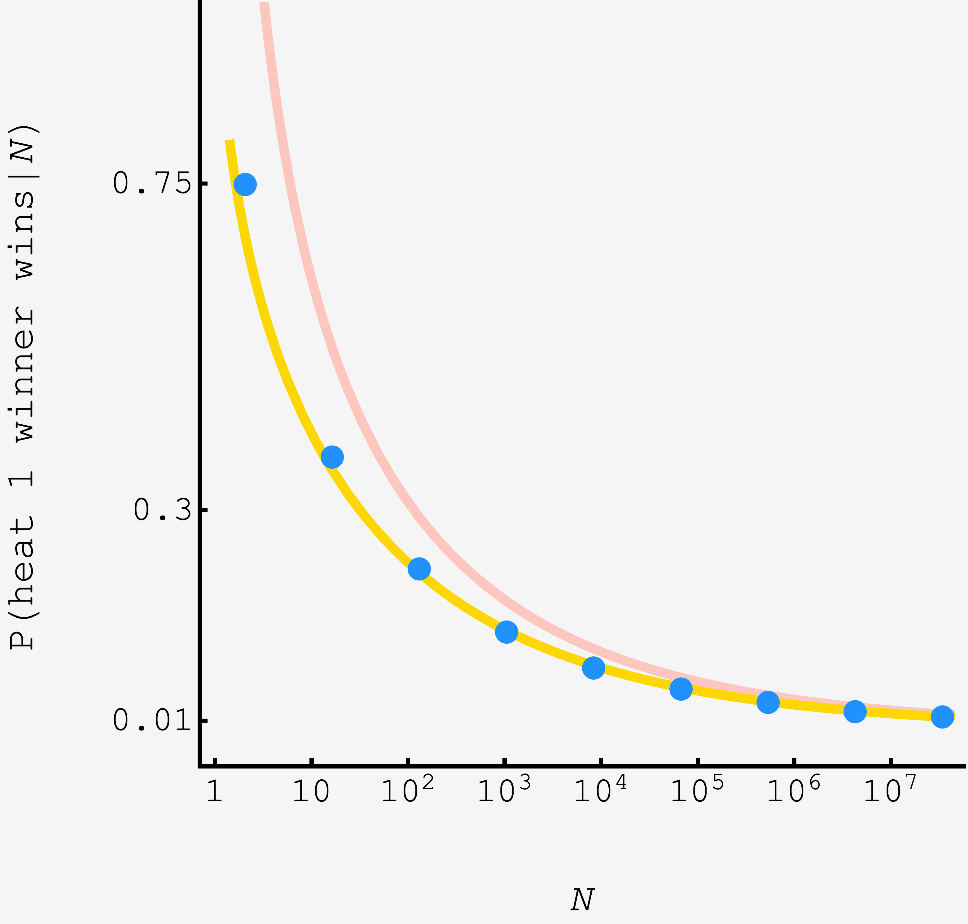
The light salmon curve shows the original model, and the gold curve shows the refined model. The fidelity at small $N$ is significantly improved, already in the ballpark for $N=2$, giving $\approx 67.9\%$ compared to the true answer of $0.75,$ and for $N=30$ gives $\approx 30.4\%$ compared to $31.5\%.$
Given the invert $\rightarrow$ scale $\rightarrow$ remap structure of the solution, we can even use it to anticipate the shape.
The $\text{erfc}^{-1}(2/N)$ piece asks “at what threshold $z$ is the tail area equal to $2/N$?,” and so returns large arguments when $N$ is large.
That answer then gets slightly more than halved by the factor $(\sqrt{2}-1)$, before the second $\text{erfc}$ asks “what is the tail area beyond this value of $N$?” with the overall effect yielding a larger small number. This is in line with the shallow decay compared to standard issue $\text{erfc}(\log N).$