Question: You and two friends have arranged to meet at a popular downtown mall between $3$ p.m. and $4$ p.m. one afternoon. However, you neglected to specify a time within that one-hour window. Therefore, the three of you will be arriving at randomly selected times between $3$ p.m. and $4$ p.m. Once each of you arrives at the mall, you will be there for exactly $15$ minutes. When the $15$ minutes are up, you leave.
At some point (or points) during the hour, there will be a maximum number of friends at the mall. This maximum could be one (sad!), two, or three. On average, what would you expect this maximum number of friends to be?
Extra Credit: Instead of three total friends, now suppose there are four total friends (yourself included). As before, you all arrive at random times during the hour and each stay for 15 minutes.
On average, what would you expect the maximum number of friends meeting up to be?
Solution
For both questions, the task at hand is enumerating how many ways there are for $1$, $2$, $3$, or $4$ friends to be at the mall at the same time, turn those descriptions into constraints on the space of arrival times ${t_1, t_2, \ldots}$, and then find the sub-volumes by integration. That’s what’s described in the first two sections below.
Extending that style of analysis to high $N$ is not simple, because the mutual constraints between the $t_j$ get complicated, as does evaluating the resulting integrals. Instead, I approximate the window of overlap as the outcome of a Poisson process, look at excitations of the window, and ask at what number of friends $k$ would we expect to see one such occurrence over the hour. This leads to a seemingly exact asymptotic formula, though as we’ll see, it is not totally justified by the analysis.
$N=3$ friends
Let $t_j$ be the time that friend $j$ arrives and $s$ the fraction of an hour that they stay for (in this case $s=\frac14$). The max can either be $1$, $2$, or $3$. If it’s $1$ then none of the friends overlap at all, and the probability is equal to
\[\begin{align} P_3(\text{max}=1) &= 3! \int\limits_0^{1-2s}\text{d}t_1 \int\limits_{t_1+s}^{1-s}\text{d}t_2 \int\limits_{t_2+s}^1\text{d}t_3 \\ &= (1-2s)^3. \end{align}\]If it’s $3$ then they all have to occur within $s$ of friend $1$’s arrival, and the probability is equal to
\[\begin{align} P_3(\text{max}=3) &= 3! \int\limits_0^1\text{d}t_1 \int\limits_{t_1}^{t_1+s}\text{d}t_2 \int\limits_{t_2}^{t_1+s}\text{d}t_3 \\ &= 3s^2. \end{align}\]Because the probabilities sum to $1$, we can figure out $P(\text{max}=2)$ and calculate the expectation
\[\begin{align} \langle \text{max}_3 \rangle &= \sum_j j \cdot P(\text{max} = j) \\ &= \left(1 + 6 s - 9 s^2 + 6 s^3\right)\bigg\rvert_{s=\frac12} \\ &=\frac{65}{32} \\ &\approx 2.03 \end{align}\]$N=4$ friends
With $4$ friends, the cases from above generalize directly, giving $P_4(\text{max}=1)=(1-3s)^4=\frac{1}{256}$ and $P_4(\text{max}=4) = (4-3s)s^3 = \frac{13}{256}$. However, we have to deal with one of the intermediate cases. We’ll go for $P(\text{max}=3).$
There are two ways to realize $\text{max}=3$. One is for three of the friends to overlap while the fourth friend overlaps with at most one of the other friends. This means
\[\begin{align} P_4(\text{one triple}) &= 2\times 4! \int\limits_0^{1-s}\text{d}t_1\,\hspace{-1em} \int\limits_{t_1}^{\min(t_1+s,1-s)}\hspace{-1em}\text{d}t_2\, \int\limits_{t_2}^{t_1+s}\text{d}t_3\, \hspace{-0.5em}\int\limits_{t_2+s}^1\text{d}t_4\, \\ &= 2s^2(6+s(11s-16)) \\ &= \frac{86}{256} \end{align}\]The other way is for there to be two distinct $3$-friend overlaps, in other words $t_3-t_1 \leq s,$ $t_4-t_2\leq s,$ while $t_4-t_1 \gt s.$ This means
\[\begin{align}P_4(\text{two triples}) &= 4! \int\limits_0^{1-s}\text{d}t_1\,\int\limits_{t_1}^{t_1+s}\text{d}t_2\, \int\limits_{t_2}^{t_1+s}\text{d}t_3\, \hspace{-0.75em}\int\limits_{\max(t_1+s,t_3)}^{\min(1,t_2+s)}\text{d}t_4\, \\ &= 4s^3-5s^4 \\ &= \frac{11}{256}\end{align}\]Putting these all together, we get
\[\begin{align} \langle \text{max}_4 \rangle &= \sum_j j \cdot P(\text{max} = j) \\&= \left(1 + 12 s - 42 s^2 + 88 s^3 - 70 s^4\right)\bigg\rvert_{s=\frac12} \\ &=\frac{317}{128} \\ &\approx 2.48 \end{align}\]General $N$ case
I now present a calculation which led to a formula that tightly captures the large $N$ behavior.
The spirit of the calculation is to find the number of overlapping friends $k$ we would expect to see once in the typical hour.
The big picture is roughly
- model each of $4$ independent intervals as a Poisson process,
- find the probability that at any given point in time, the window would have $k$ friends, then
- compute the $k$ at which we would expect one such interval to spawn per hour
Let’s assume there are $1/s = 4$ effectively independent intervals. The rate at which the friends arrive is $\lambda = N\,\text{hr}^{-1}$, so the probability that nobody shows up in time $\Delta t$ is $(1-\lambda \Delta t)$ and the chance nobody shows up for time $t$ is $(1-\lambda \Delta t)^{t/\Delta t}$ which becomes $e^{-\lambda t}$ as $\Delta t$ goes to zero. The probability that someone shows up in time $dt$ is $\lambda dt$ so the chance that $k$ people show up in time $T$ is (making aggressive assumption $\lambda$ stays constant) approximately
\[\begin{align} P(k\,\,\text{friends in time}\,\, T) &\approx \int \lambda\, dt_1 \int \lambda\, dt_2 \ldots \int \lambda\, dt_k\, e^{-\lambda(t_1 + t_2 + \ldots + t_k)} \\ &= \lambda^k e^{-\lambda s} \int\, dt_1 \int\, dt_2 \ldots \int\, dt_k \\ &= \frac{(\lambda s)^k}{k!} e^{-\lambda s}, \end{align}\]a Poisson distribution. The expectation of this distribution is $\mu = \lambda s = N s$ and is approximately Gaussian for large $N.$ So
\[P(\text{max}=k) = \frac1{k!} \mu^k e^{-\mu }\]If we take the logarithm, then we get
\[\begin{align} \log P(\text{max} = k) &= k\log \mu - \mu - \log k! \\ &= k\log\mu - \mu - \left(k\log k - k + \frac12 \log 2\pi k\right) \end{align}\]We want to see the behavior around the mean, so we can center about $\mu = k - \delta$ and expand the $\log$ terms
\[\begin{align}\log P(\text{deviation} = \delta) &= \delta + (\mu + \delta) \log\mu - (\mu + \delta)\log(\mu + \delta) - \frac12\log 2\pi(\mu+\delta) \\ &= \delta - (\mu + \delta) \log\frac{\mu + \delta}{\mu} - \frac12\log 2\pi(\mu+\delta) \\ &= \delta - (\mu + \delta) \log\left(1 + \delta/\mu\right) - \frac12\log 2\pi(\mu+\delta) \\ &= \delta -(\mu+\delta)\left(\delta/\mu - \frac12\delta^2/\mu^2\right) - \frac12\log 2\pi(\mu+\delta) \\ &= \delta - \delta + \frac12 \delta^2/\mu - \delta^2/\mu + \frac12\delta^3/\mu^2 - \frac12\log 2\pi(\mu+\delta) \\ &\approx -\frac12\delta^2/\mu - \frac12\log 2\pi\mu\end{align}\]So, exponentiating the probability, the chance of seeing a deviation of size $\delta$ at a random point in time is approximately
\[P(\delta) = \frac{1}{\sqrt{2\pi\mu}}\large e^{-\frac12\delta^2/\mu}\]The probability that a random time is inside an excitation of magnitude $\delta$ is equal to the rate at which such intervals spawn times the amount of time they last once they exist
\[P(\delta) = r(\delta)\tau(\delta).\]The expected maximum magnitude of excitation $\delta$ is the interval whose spawn rate is exactly once per hour, so
\[P(\delta) = \tau(\delta)\]We treat the interval whose default state is to have the average number of friends $\mu = Ns$ and keep track of the friends who come or go. We need to find the lifetime of an excitation of magnitude $\delta = k-\mu.$ If there are $\delta$ excess friends in the excitation, they all spawned with the window size $s$ of one another, so we’d expect the oldest friend to have time $s/\delta$ remaining before they leave the window.
Plugging this into the last equation, we get
\[s/\delta = \frac{1}{\sqrt{2\pi\mu}}e^{-\frac12\delta^2/\mu}.\]This equation can’t be solved outright for $\delta$, but we can use it to develop an approximation. Taking logs we get
\[\log\frac1s = \frac12\delta^2/\mu + \log\sqrt{2\pi\mu} - \log\delta.\]We’re about to see the unjustified step.
The thinking goes roughly: $\log\frac1s$ doesn’t grow at all, so the right side mustn’t either. However, the second term grows as $\log\sqrt{\mu}$, so the negative term must also grow as $\log\sqrt{\mu},$ since the $\delta^2/\mu$ term is positive.
Therefore, to leading order we have $\log\frac1s \approx \frac12\delta^2/\mu$ and $\delta = \sqrt{2\mu\log\frac1s}$ leading to
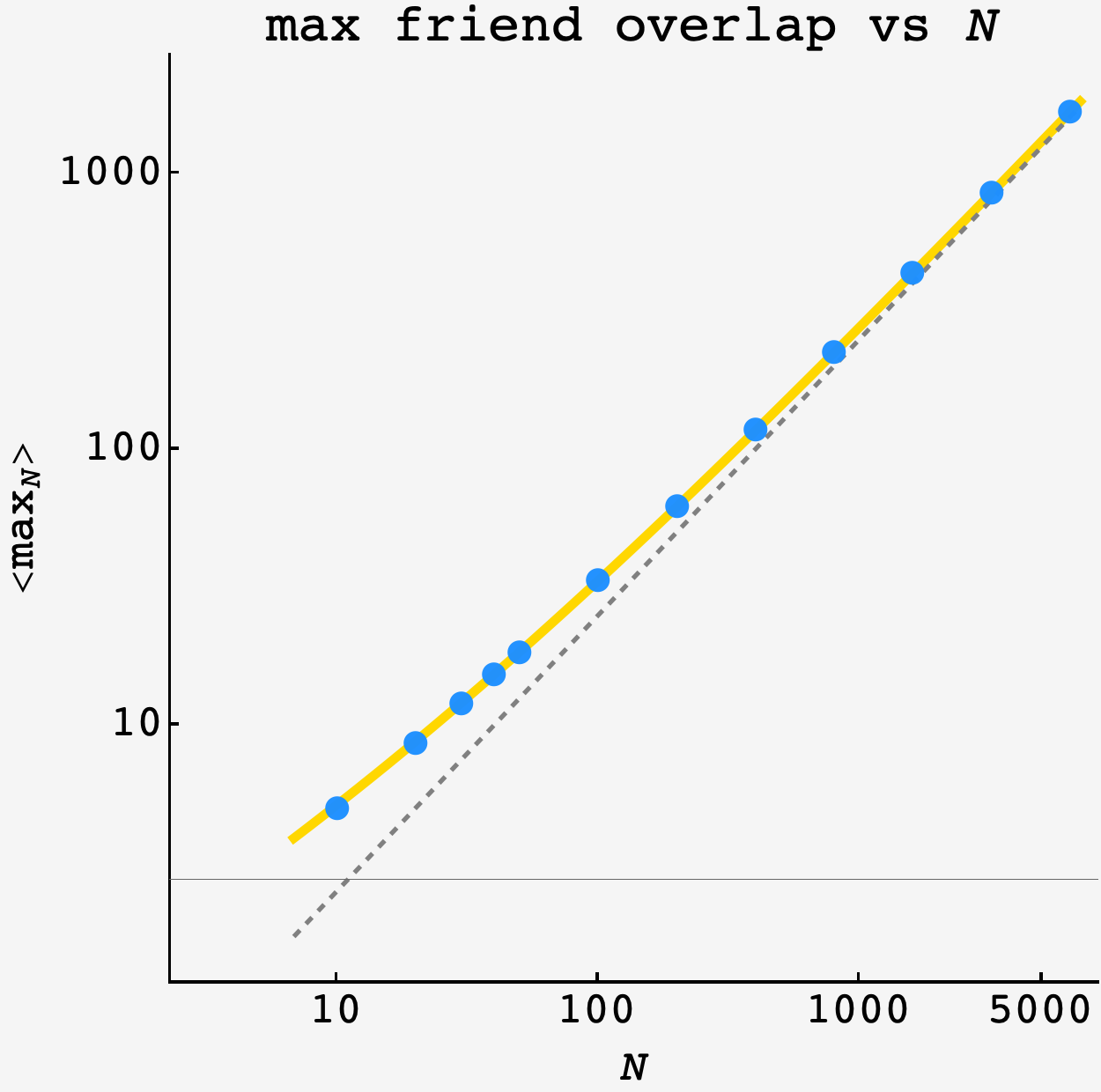
\[\begin{align} k &= \mu + \delta \\ &= Ns + \sqrt{2Ns\log\frac1s}\end{align}.\]This is a wonderful formula that closely matches the data as $N$ scales:
However, $\delta = \sqrt{2\mu\log\frac1s}$ is not a close approximation for the numerical solution of the $P(\delta) = \tau(\delta)$ equation.
In the first place, we know that we’re making an aggressive assumption (that the intervals are Poisson processes with a rate $\lambda$ that remains constant as friends come and go, even though we should expect it to rise or fall as we observe windows of low or high friend attendance). So, we shouldn’t expect the numerical solution to be a perfect model for $\delta.$ In fact, we should expect to underestimate the extrema with this approach, since $\lambda$ doesn’t deplete after a large excitation or build after gaps of no arrivals.
By ignoring the normalization of the probability distribution and the term $\delta$ from the estimation of the excitation lifetime, we make a correction in the other direction, forcing $\delta$ to be bigger before the two sides balance.
However, there’s no good reason to suspect this double error to make the prediction spot-on.
In the time I had, I did not arrive at a more fundamental path to this result, though it demands sound explanation.