Can you permeate the bipyramid?

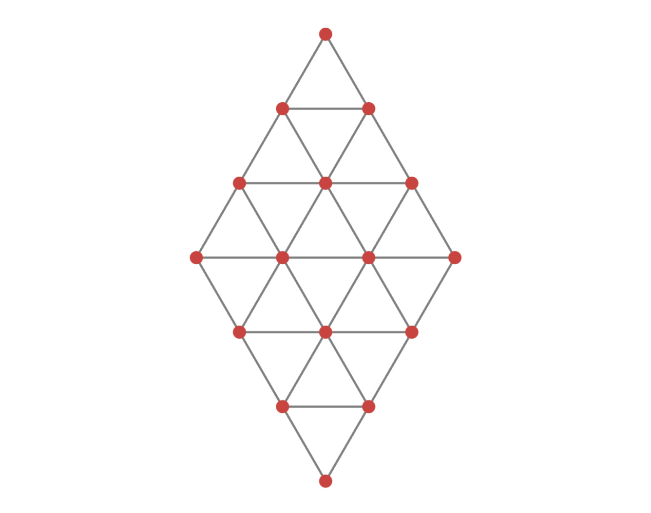
Question: Consider the following figure, which shows 16 points arranged in a rhombus shape and connected to their neighbors by edges. How many distinct paths are there from the top point to the bottom along the edges such that:

• You never visit the same point twice.
• You only move downward or sideways—never upward.

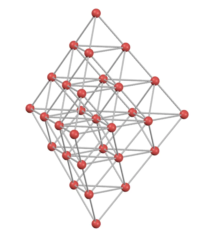
Extra credit: Consider the following figure, which shows $30$ points arranged in a three-dimensional triangular bipyramid. As before, points are connected to their neighbors by edges. How many distinct paths are there from the top point to the bottom along the edges such that:

• You never visit the same point twice.
• You only move downward or sideways—never upward.

(Fiddler on the Proof)

Solution

The standard problem can be done analytically, but setting it up is nearly the same as the extra credit, which can’t. We’ll do the computational approach first.

First of all, give each layer a label $\ell.$ Each path enters layer $\ell$ at a node $j$ from one of its neighbors in layer $(\ell-1).$

Call $\Omega(i, \ell)$ the number of ways to arrive at node $i$ as the last node you visit in layer $\ell,$ $W(j, \ell)$ the number of ways to arrive at node $j$ as the first node you visit in layer $\ell,$ and $T(i\leftarrow j, \ell)$ the number of ways to travel from node $j$ to node $i$ staying entirely within layer $\ell$ and not revisiting any nodes.

Any path that leaves layer $\ell$ at node $i$ enters layer $\ell$ at some other node $j$ then travels to $i,$ so

Putting this to code, we have

def omega(n):
  
  if n.layer == 0:
    return 1

  return sum(
      T(n, j) * W(j) for j in layer_of(n)
    )

Also, the number of ways to arrive at node $i$ as the first node visited in layer $\ell$ is equal to sum over ways to exit layer $(\ell-1)$ from one of the neighbors of $i$ (in layer $(\ell-1)$), so

In code, we have

def W(j):

  return sum(
      omega(n) for n in vert_neighbors(j)
  )

In the standard puzzle, $T(i\leftarrow j, \ell)$ is simply $1$ since there is one path from each node in a layer to another node in the layer. In the $3\text{D}$ problem, we need to search to find the number of paths from node $j$ to node $i$ within a layer.

def T(i, j):
  # for the standard problem, just return 1

  visited = frozenset([i])

  def find_T(i, j, visited):

    neighbors = layer_neighbors(i)
    neighbors = [ n for n in neighbors if n not in visited ]

    if i == j: 
      return 1
    if not neighbors: 
      return 0

    return sum(
          find_T(n, j, visited.union({n})) 
            for n in neighbors
    )
    
  return find_T(i, j, visited)

In the code above, we’re using $i$ and $j$ to refer to nodes, but really we need three labels to specify a node in the $3D$ problem, its layer $\ell$, and its coordinates within its layer. Since each layer is a triangle, we can designate one corner of the triangle as row zero, and measure the other nodes in terms of their row (perpendicular distance from the zero corner), and their index (distance from the left edge of the triangle).

In this scheme, the node at the zero corner in any layer is $(0,0,\ell)$, the corner in the bottom left is $(\ell,0,\ell)$ and the corner in the bottom right is $(\ell,\ell,\ell).$

We need lookups that store the neighbors of a node within its layer, as well as its vertical neighbors. Overlaying one layer of the grid on the next, we see that in the upper bipyramid, the candidate vertical neighbors of a node $(r, i, \ell)$ are $\{(r,i,\ell-1),(r-1,i,\ell-1),(r-1,i-1,\ell-1)\},$ filtered for any points that fall outside the confines of the grid. Going down it’s the same with the row and index shifts reversed: $\{(r,i,\ell-1),(r+1,i,\ell-1),(r+1,i+1,\ell-1)\}.$

def vert_neighbors(n):
  if n.layer == 0:
    return []
  
  else:
    if n.layer < (L + 1) // 2:

      if n.index > n.row or n.row > n.layer:
        return []

      candidates = [ Node(n.row, n.index, n.layer - 1)
                   , Node(n.row - 1, n.index, n.layer - 1)
                   , Node(n.row - 1, n.index - 1, n.layer - 1)
                   ]

      filtered = [ c for c in candidates 
                  if 0 <= c.index <= c.row and c.row <= c.layer
                 ]
    
    else:
      if n.index > n.row or n.row > L - n.layer - 1:
        return []

      candidates = [ Node(n.row, n.index, n.layer - 1)
                   , Node(n.row + 1, n.index, n.layer - 1)
                   , Node(n.row + 1, n.index + 1, n.layer - 1)
                   ]

      filtered = [ c for c in candidates 
                  if 0 <= c.index <= c.row and c.row < L - c.layer 
                 ]
    
    return filtered

Within a layer, the neighbors for an interior point are just the nearest neighbors on the hexagonal lattice, filtered for actually being inside the confines of the pyramid:

def layer_neighbors(n):
  candidates = [ Node(n.row - 1, n.index, n.layer)
               , Node(n.row - 1, n.index - 1, n.layer)
               , Node(n.row, n.index - 1, n.layer)
               , Node(n.row, n.index + 1, n.layer)
               , Node(n.row + 1, n.index, n.layer)
               , Node(n.row + 1, n.index + 1, n.layer)
               ]

  row_upper_bound = n.layer if n.layer < L / 2 else L - n.layer - 1

  filtered = [ c for c in candidates 
              if 0 <= c.index <= c.row and 0 <= c.row <= row_upper_bound
             ]

  return filtered

Finally, we have a function that returns all points of a given layer, used for the in-layer path searching:

def layer_of(n):

  upper_bound_rows = n.layer if n.layer < L / 2 else L - n.layer - 1

  nodes = [ Node(r, j, n.layer)
                for r in range(upper_bound_rows + 1)
                  for j in range(r + 1)
             ]

  return nodes

For clarity, nodes were implemented as named tuples like so:

from collections import namedtuple
Node = namedtuple('Node', ['row', 'index', 'layer'])

With this program in hand, we can run it for the $3\text{D}$ bipyramid which gets $1,093,007,025$ distinct paths.

Making alterations to the code for $T$, and the neighbors, we get $2,304$ paths for the $2\text{D}$ case.

Analytic solution for standard question

The in-layer side steps connect pairs of layer nodes with unique straight-line paths, so they don’t actually increase the multiplicity. As a result, the overall number of paths is just the product of downward paths available at each level. Two edges emerge from every node, so for the problem at hand this is (as we found above)

and in general it becomes