Can you witness an epic collapse?

Question:If you follow the NBA, then you probably know Boston Celtics had several improbable comebacks against the Indiana Pacers in this year’s playoffs. But given that the Pacers had a “$90$ percent chance or higher” to win at some point in a game, did that mean their probability of winning that game was actually $90$ percent?

Let’s explore this with a toy (i.e., simplified) version of basketball.

Suppose you’re playing a game in which there are five “possessions.” For each possession, there’s a $50$ percent chance that your team scores one point. If you don’t score, then your opponent instead scores one point.

After the game, ESPN reports that your opponent’s chances of winning were “$75$ percent chance or higher” at some point during the game (i.e., before the final possession is complete).

Given this information, what was the probability that your team actually won the game?

For Extra Credit, instead of five possessions, now suppose there are $101$. Again, with each possession, there’s a $50$ percent chance that your team scores one point. If you don’t score, then your opponent instead scores one point.

After the game, ESPN reports that your opponent’s chances of winning were “$90$ percent chance or higher” at some point during the game (i.e., before the final possession is complete).

Given this information, what was the probability that your team actually won the game?

(Fiddler on the Proof)

Solution

We’re interested in collapses:

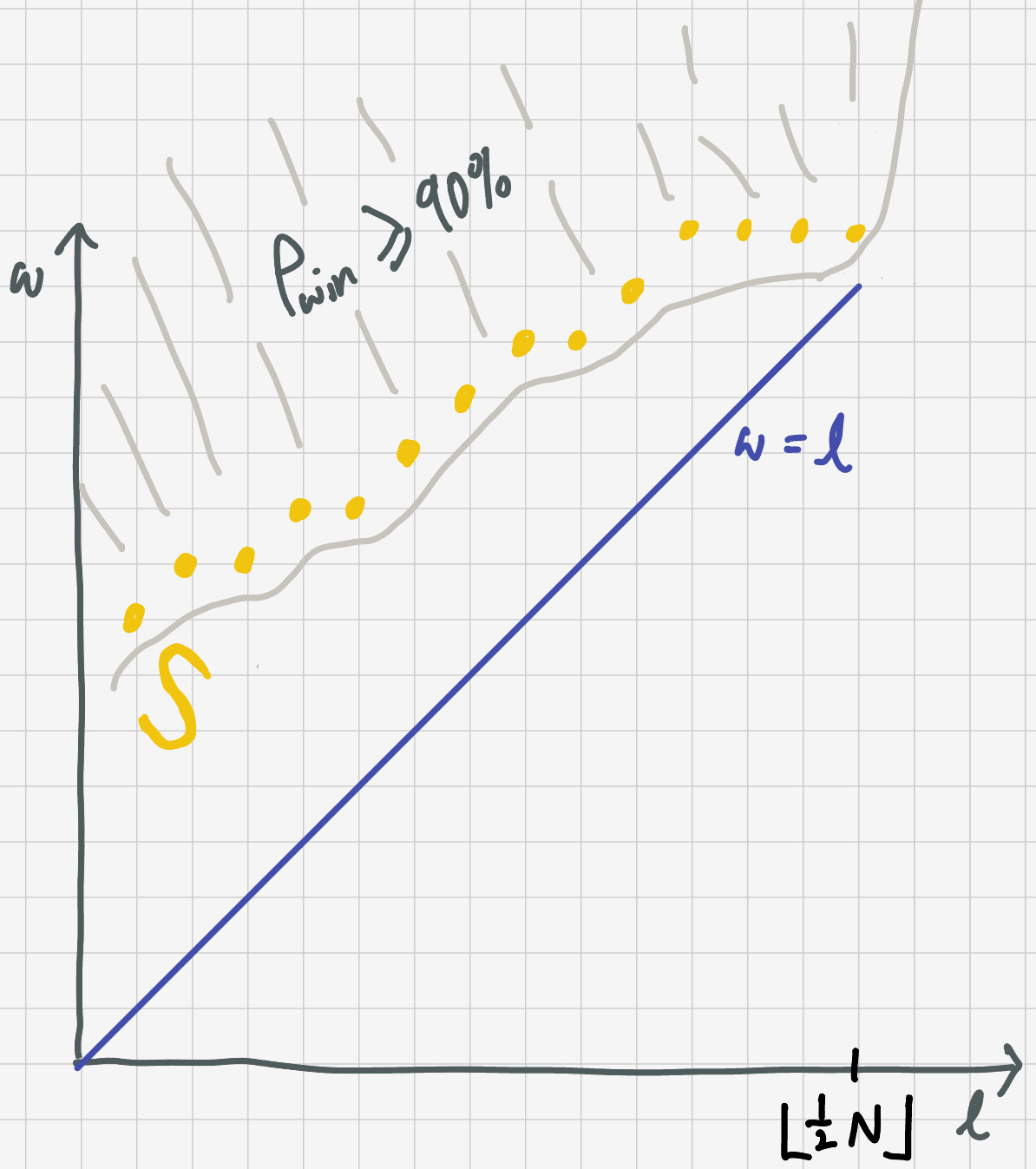
The probability of winning a game is a function of the possessions that already happened, and the number of possessions that remain. Intuitively, to get a $90\%$ win probability early in the game requires a bigger lead than later in the game.

The set of game states with $P_\text{win} \geq 90\%$ form a region in $(\ell, w)$-space where $w$ is the number of possessions the team has won and $\ell$ is the number they’ve lost. The boundary of this region forms a set of boundary points $\mathcal{S}.$

If we can find the probability of arriving at each point $S_i$ in $\mathcal{S},$ $P(\text{start} \rightarrow S_i)$ and the probability to lose after getting there $P(S_i\rightarrow\text{lose})$ then we can find the overall probability of seeing a team collapse:

To avoid double counting, $P(\text{start}\rightarrow S_i)$ should be the “first passage” probabilities to the set $\mathcal{S}.$ In other words, the probability that the game reaches the state $S_i$ without visiting another point in $\mathcal{S}$ before. Were we to include second visitations, that would mean that a game could reach the $\geq 90\%$ region, then leave it, then come back, then collapse, and it would count twice toward being a collapse.

So, we modify our equation

We can find the first passage probability to a state $S_i \in \mathcal{S}$ by finding the unconditional probability to arrive there, and then subtracting off the probability of going there by way of any earlier point $S_j \in \mathcal{S}.$

The probability of going to $S_i$ via $S_j$ is just $P_\text{first passage}(\text{start} \rightarrow S_j) P(S_j \rightarrow S_i),$ so we get the recursive relationship

The base case is the number of ways to get to the first point of the boundary $S_1,$ for which the sum term is zero.

To lose a game, the team needs to finish the game with $\lfloor \frac12 N\rfloor + 1$ total losses. So, to lose the game from state $(\ell, w)$ the team need at least $\lfloor \frac12 N\rfloor + 1 - \ell$ additional losses from here on out. If they lose more, that’s great, and they can lose up to $N - (w + \ell)$ additional possessions.

We can visualize the end game like so:

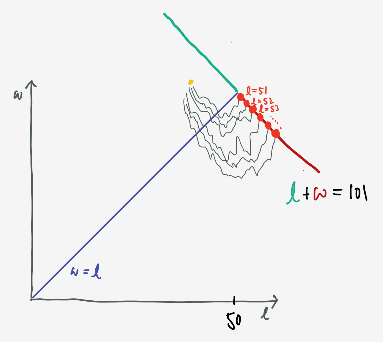
Finishing anywhere on the green segment is a win, and anything on the red a loss.

If the game is at point $(\ell, w)$ we need to count how many ways there are to end up on the red segment:

The probability of moving from a point $(\ell_1, w_1)$ to point $(\ell_2, w_2)$ is the number of ways to order $(w_2-w_1)$ wins and $(\ell_2-\ell_1)$ losses, times the probability of choosing any one of those orders:

The last piece we need is the actual set of points $\mathcal{S}.$ We could find it by scanning all $(\ell, w)$ and testing whether the formula for $P_\text{loss}$ is less than $(1 - 0.9) = 0.1,$ then find the lowermost points of the set, however this is quadratic in $N.$

We can be a little bit smarter by starting at $(\ell, w) = (0,0)$ and increasing $w$ until $P_\text{lose}(\ell, w) \lt 0.1.$ We then increase $\ell$ by $1$ and again increase $w$ until $P(\ell+1, w) \lt 0.1$ and so on and so forth.

We can implement this in Python to find the boundary like so:

from scipy.special import comb as binom
from functools import lru_cache

N = 101

@lru_cache(maxsize=None)
def P_transit(Si):
  l, w = Si

  return 1 / 2.0 ** (w + l) * binom(w + l, w, exact=True)
  

@lru_cache(maxsize=None)
def P_to_lose(Si, N):
    l, w = Si
    P = 0

    # HAVE TO LOSE AT LEAST (floor(N/2) + 1 - l) MORE TIMES
    min_losses = N // 2 + 1 - l
    max_losses = N - (w + l)

    for losses in range(min_losses, max_losses + 1):
        wins = N - (w + l) - losses
        S_temp = (wins, losses)
        P += P_transit(S_temp)

    return P

# FIND THE POINTS OF S
w = 0
S_frontier = []

for l in range(0, N // 2):

  while P_to_lose((l, w), N) > 0.1:
    w += 1

  S_frontier += [(l, w)]

With the frontier in hand, we can calculate the first passage probabilities:

def tuple_minus(a, b):

  return (a[0] - b[0], a[1] - b[1])

@lru_cache(maxsize=None)
def P_fp(Si):

  P_repeat_visit = sum(
                        P_fp(Sj) * P_transit(tuple_minus(Si, Sj))
                        for Sj in S_frontier if Sj[0] < Si[0]
                      )

  return P_transit(Si) - P_repeat_visit

And finally, calculate the probability of witnessing a collapse:

P_collapse = sum( P_fp(Si) * P_to_lose(Si, N) for Si in S_frontier )

which comes to about $P_\text{collapse} \approx 0.039818127\ldots$

If we condition on the news that the team had a $90\%$ chance to win (i.e. they reached $\mathcal{S}$ at some point), then we get

P_collapse_after_news = P_collapse / sum( P_fp(Si) for Si in S_frontier )

which is about $P_\text{collapse after news} \approx 0.07741987677639166\ldots$