Question: Once again, I’m painting an infinitely long strip of canvas, broken up into adjacent $1$ cm-by-$1$ cm squares. Squares are randomly and independently numbered $0$ or $1.$ But this time, the strip itself is $2$ cm wide.
Squares are considered adjacent if they share a common edge. So squares can be horizontally or vertically adjacent, but not diagonally adjacent.
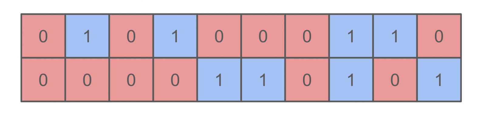
Once I’m done painting, there will again be many “clusters” of contiguous red and blue squares. The example below contains $20$ total squares and nine clusters, which means the average size of a cluster here is approximately $2.22$ squares.
Once I’m done painting, what will be the average size of each red or blue cluster?
Solution
Outline
To make a cluster with $s$ tiles, we need all $s$ of those tiles to be one color, and all of the tiles on the perimeter to be another. So, the probability of any given configuration is just $q^s(1-q)^p$. also, the configuration might have a $2$ or $4$-fold symmetry.
Given these configurations, finding their probability is straightforward. However, getting the configurations is not and, so, will spoil an exact calculation.
The big idea of this solution is to find the configurations for the first few cluster sizes, and observe how successive generations are formed from earlier ones. This motivates a simplifying assumption, that for large cluster sizes $s,$ the probabilities start to follow a geometric series. With this assumption, we’ll build a model that gets the ratio of subsequent probabilities and with this approximate probability distribution, we’ll calculate the average cluster size.
Configuration inspection
To start, let’s analyze the configurations for the first few cluster sizes.
For $s=1$ we have a single tile colored opposite from its three nearest neighbors. Also, we can place the tile in the top or bottom row. So, the relative frequency of $s=1$ tiles is
\[P(1) = 2q(1-q)^3.\]For $s=2$ we can place two tiles horizontally or vertically. In either case there are $4$ perimeter tiles. In the case of the horizontal tile, we can put it in the top or bottom row. The relative frequency of $s=2$ tiles is therefore
\[P(2) = 3q^2(1-q)^4.\]For $s=3$ we can have a row of $3$ with $5$ nearest neighbors or a right angle arrangement with $4$ neighbors. The row has degeneracy $2$ and the right angle has degeneracy $4$. Putting it together, the relative frequency is
\[P(3) = 2q^3(1-q)^5 + 4q^3(1-q)^4.\]For $s=4$ there are more exotic arrangements, which we’ll draw (below) without talking through. Translating the drawings into probabilities with the same reasoning as above, we get
\[P(4) = 2q^4(1-q)^6 + 5q^4(1-q)^4 + 4q^4(1-q)^5.\]How’s it growing?
If we draw out each collection of configurations, and how they lead to the next collection, we can see there is a lot of mixing going on. And, apart from the pipes, there are not really cleanly separable lineages.

This makes it reasonable to think that each generation leads to the next as a conglomerate. In a loose sense, the collections of clusters of size $s$ forms a surface in “shape space” and the next generation of clusters of size $(s+1)$ is formed by branching off that surface.
Further, there isn’t a strong reason to expect the decay between steps to depend strongly on $s$ since the extension of an $(s-1)$ cluster into an $s$-cluster depends on local, single site attachments.
If we plug the value of $q$ into the expression above, they become $P_2 = \frac38 P_1,$ $P_3 = \frac56 P_2,$ and $P_3 = \frac34 P_4.$ These ratios are approximately $0.38,$ $0.83,$ and $0.75.$ if we carry out the next few, we get $0.69,$ $0.73,$ $0.71,$ and $0.72.$
It seems like these numbers are settling down to a value near $0.72,$ in support of the conglomerate view.
Self-consistent dominoes
In this spirit, let’s write down a model relating the probability of size $s$ clusters to the probability of size $(s-1)$ clusters. We’ll envision a growth process where we build clusters left to right, laying down dominoes one at a time. The dominoes can either be both red, red on top and blue on bottom, or blue on top and red on bottom and we’ll track which domino each cluster ends in. For ease of rendering, we’ll consider the cluster color to be filled-in squares, and the opposite color to be empty squares.
If we have a cluster of size $s$ ending in ${\square \atop \blacksquare}$ it could be built either from a $(s-1)$-sized cluster ending in ${\square\atop\blacksquare}$ or ${\blacksquare\atop\blacksquare}$ and each additional domino has probability $\frac14$ to be drawn:
\[P\left(s, {\square \atop \blacksquare}\right) = \frac14P\left(s-1, {\square \atop \blacksquare}\right) + \frac14 P\left(s-1, {\blacksquare \atop \blacksquare}\right).\]Because the top and bottom row are symmetric, the same equation governs clusters ending in ${\blacksquare\atop\square}:$
\[P\left(s, {\blacksquare \atop \square}\right) = \frac14P\left(s-1, {\blacksquare \atop \square}\right) + \frac14 P\left(s-1, {\blacksquare \atop \blacksquare}\right).\]If a cluster ends in ${\blacksquare\atop\blacksquare}$ it could have come from a cluster ending in ${\blacksquare\atop\blacksquare}$, ${\square\atop\blacksquare}$, or ${\blacksquare\atop\square},$ which would have had size $(s-2)$ so
\[P\left(s, {\blacksquare \atop \blacksquare}\right) = \frac14P\left(s-2, {\blacksquare \atop \square}\right) + \frac14P\left(s-2, {\square \atop \blacksquare}\right) + \frac14 P\left(s-2, {\blacksquare \atop \blacksquare}\right).\]Now, by our assumption, the probability of a cluster of size $s$ is some constant factor times the probability of a cluster of size $(s-1)$ or $P(s)=\gamma P(s-1).$ Plugging this into the first equation, we get
\[P\left(s, {\square \atop \blacksquare}\right) = \frac1{4\gamma}P\left(s, {\square \atop \blacksquare}\right) + \frac1{4\gamma} P\left(s, {\blacksquare \atop \blacksquare}\right)\]which we can solve to get
\[P\left(s, {\square \atop \blacksquare}\right) = \dfrac{1}{4\gamma-1}P\left(s, {\blacksquare \atop \blacksquare}\right),\]with the same kind of relationship holding for $P\left(s,{\blacksquare\atop\square}\right).$
We can plug both of these into the equation for $P(s,{\blacksquare\atop\blacksquare})$ to get
\[P\left(s,{\blacksquare\atop\blacksquare}\right) = \left(\frac1{2\gamma^2}\frac{1}{4\gamma-1} + \frac1{4\gamma^2}\right)P\left(s,{\blacksquare\atop\blacksquare}\right)\]which is only true if the expression in $\gamma$ is equal to $1.$ Solving $\displaystyle\frac1{2\gamma^2}\frac{1}{4\gamma-1} + \frac1{4\gamma^2} - 1 = 0$ we find a single real root at $\gamma \approx 0.71878\ldots$
Expected cluster size
Under our assumption, the likelihoods for large clusters follow a geometric series with relative factor $\gamma.$ So, we can calculate exact probabilities up to some cluster size $s^*$ and replace all further terms with $\gamma P(s^*),$ $\gamma^2 P(s^*)$ and so on.
Given our work above, we can cavalierly choose $s^*=4,$ and the expected cluster size becomes
\[\begin{align} \langle s\rangle &= \dfrac{\sum\limits_{s=0}^\infty s P(s)}{\sum\limits_{s=0}^\infty P(s)} \\ &\approx \dfrac{P(1) + 2P(2) + 3P(3) + P(4)\left(4 + 5\gamma + 6\gamma^2 + \ldots\right)}{P(1) + P(2) + P(3) + P(4)\left(1 + \gamma + \gamma^2 + \ldots\right)} \\ &\approx 3.198\ldots \end{align}\]which matches simulation.